Rigidbody

Rigidbody#

class c4dynamics.states.lib.rigidbody.rigidbody(x=0, y=0, z=0, vx=0, vy=0, vz=0, phi=0, theta=0, psi=0, p=0, q=0, r=0)[source]#

A rigid-body object

The rigidbody extends the datapoint class to form an elementary rigidbody object in space, i.e. an object with length and attitude.

It introduces attributes related to rotational dynamics, such as angular position, angular velocity, and moment of inertia. As such its state vector consists of the following variables:

\[X = [x, y, z, v_x, v_y, v_z, \varphi, \theta, \psi, p, q, r)]^T\]

Position coordinates, velocity coordinates.
Angles, angular rates.

Arguments

xfloat or int, optional: The x-position of the datapoint. Default value \(x = 0\).
yfloat or int, optional: The y-position of the datapoint. Default value \(y = 0\).
zfloat or int, optional: The z-position of the datapoint. Default value \(z = 0\).
vxfloat or int, optional: Component of velocity along the x-axis. Default value \(v_x = 0\).
vyfloat or int, optional: Component of velocity along the y-axis. Default value \(v_y = 0\).
vzfloat or int, optional: Component of velocity along the z-axis. Default value \(v_z = 0\).
phifloat or int, optional: Euler angle representing rotation around the x-axis (rad). Default value \(\varphi = 0\).
thetafloat or int, optional: Euler angle representing rotation around the y-axis (rad). Default value \(\theta = 0\).
psifloat or int, optional: Euler angle representing rotation around the z-axis (rad). Default value \(\psi = 0\).
pfloat or int, optional: Angular rate around the x-axis (roll). (rad/sec). Default value \(p = 0\).
qfloat or int, optional: Angular rate around the y-axis (pitch). (rad/sec). Default value \(q = 0\).
rfloat or int, optional: Angular rate around the z-axis (yaw). (rad/sec). Default value \(r = 0\).

The input arguments determine the initial values of the instance. The vector of initial conditions can be retrieved by calling rigidbody.X0:

>>> from c4dynamics import rigidbody

>>> rb = rigidbody(z = 1000, theta = 10 * c4d.d2r, q = 0.5 * c4d.d2r)
>>> rb.X0 
[0  0  1000  0  0  0  0  0.174  0  0  0.0087  0]

When the initial values are not known at the stage of constructing the state object, it’s possible to pass zeros and override them later by direct assignment of the state variable with a 0 suffix. See more at state.X0.

Parameters:

mass (float) – The mass of the datapoint
I ([float, float, float]) – An array of moments of inertia

See also

lib, rotmat, state, eqm

Example

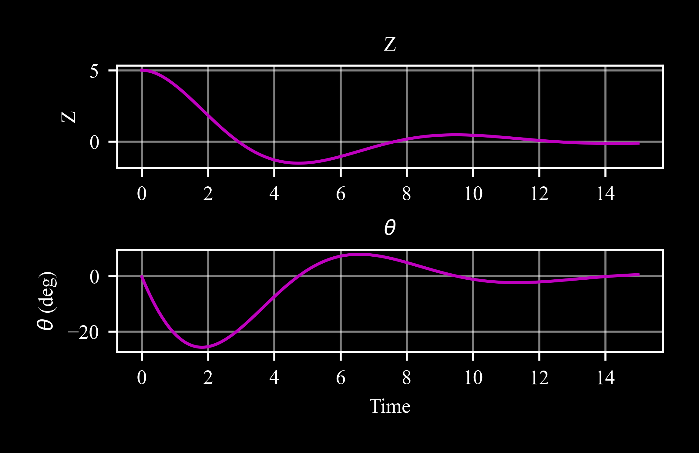
A simplified model of an aircraft autopilot is given by:

\[ \begin{align}\begin{aligned}\dot{z}(t) = 5 \cdot \theta(t)\\\dot{\theta}(t) = -0.5 \cdot \theta(t) - 0.1 \cdot z(t)\end{aligned}\end{align} \]

Where:

\(z\) is the deviation of the aircraft from the required altitude
\(\theta\) is the pitch angle

The aircraft is represented by a rigidbody object. scipy’s odeint is employed to solve the dynamics equations and update the state vector X.

import required packages:

>>> import c4dynamics as c4d
>>> from matplotlib import pyplot as plt
>>> from scipy.integrate import odeint
>>> import numpy as np

Settings and initial conditions:

>>> dt, tf = 0.01, 15
>>> tspan = np.arange(0, tf, dt)
>>> A = np.zeros((12, 12))
>>> A[2, 7] =  5
>>> A[7, 2] = -0.1
>>> A[7, 7] = -0.5
>>> f16 = c4d.rigidbody(z = 1, theta = 0)
>>> for t in tspan:
...   f16.X = odeint(lambda y, t: A @ y, f16.X, [t, t + dt])[-1]
...   f16.store(t)

>>> _, ax = plt.subplots(2, 1)
>>> f16.plot('z', ax = ax[0])   
>>> ax[0].set(xlabel = '')  
>>> f16.plot('theta', ax = ax[1], scale = c4d.r2d)
>>> plt.show()

The animate method allows the user to play the attitude histories given a 3D model (requires installation of open3D).

The model in the example can be fetched using the c4dynamics datasets module (see c4dynamics.datasets):

>>> modelpath = c4d.datasets.d3_model('f16')
Fetched successfully

>>> f16colors = np.vstack(([255, 215, 0], [255, 215, 0], [184, 134, 11], [0, 32, 38], [218, 165, 32], [218, 165, 32], [54, 69, 79], [205, 149, 12], [205, 149, 12])) / 255
>>> f16.animate(modelpath, angle0 = [90 * c4d.d2r, 0, 180 * c4d.d2r], modelcolor = f16colors)

Properties

`rigidbody.mass`	Gets and sets the object's mass.
`rigidbody.I`	Gets and sets the array of moments of inertia.
`rigidbody.angles`	Returns an array of Euler angles.
`rigidbody.ang_rates`	Returns an array of angular rates.
`rigidbody.BR`	Returns a Body-from-Reference Direction Cosine Matrix (DCM).
`rigidbody.RB`	Returns a Reference-from-Body Direction Cosine Matrix (DCM).

Methods

`rigidbody.inteqm`(forces, moments, dt)	Advances the state vector, `rigidbody.X`, with respect to the input forces and moments on a single step of time, dt.
`rigidbody.plot`(var[, scale, ax, filename, ...])	Draws plots of trajectories or variable evolution over time.
`rigidbody.animate`(modelpath[, angle0, ...])	Animate a rigidbody.

Rigidbody

Contents

Rigidbody#