c4dynamics.states.lib.rigidbody.rigidbody.I

property rigidbody.I

Gets and sets the array of moments of inertia.

\[I = [I_{xx}, I_{yy}, I_{zz}]\]

Default: \(I = [0, 0, 0]\)

Parameters:

I (numpy.array or list) – An array of three moments of inertia about each one of the axes \(([I_{xx}, I_{yy}, I_{zz}])\).

Returns:

out (numpy.array) – An array of the three moments of inertia \([I_{xx}, I_{yy}, I_{zz}]\).

Example

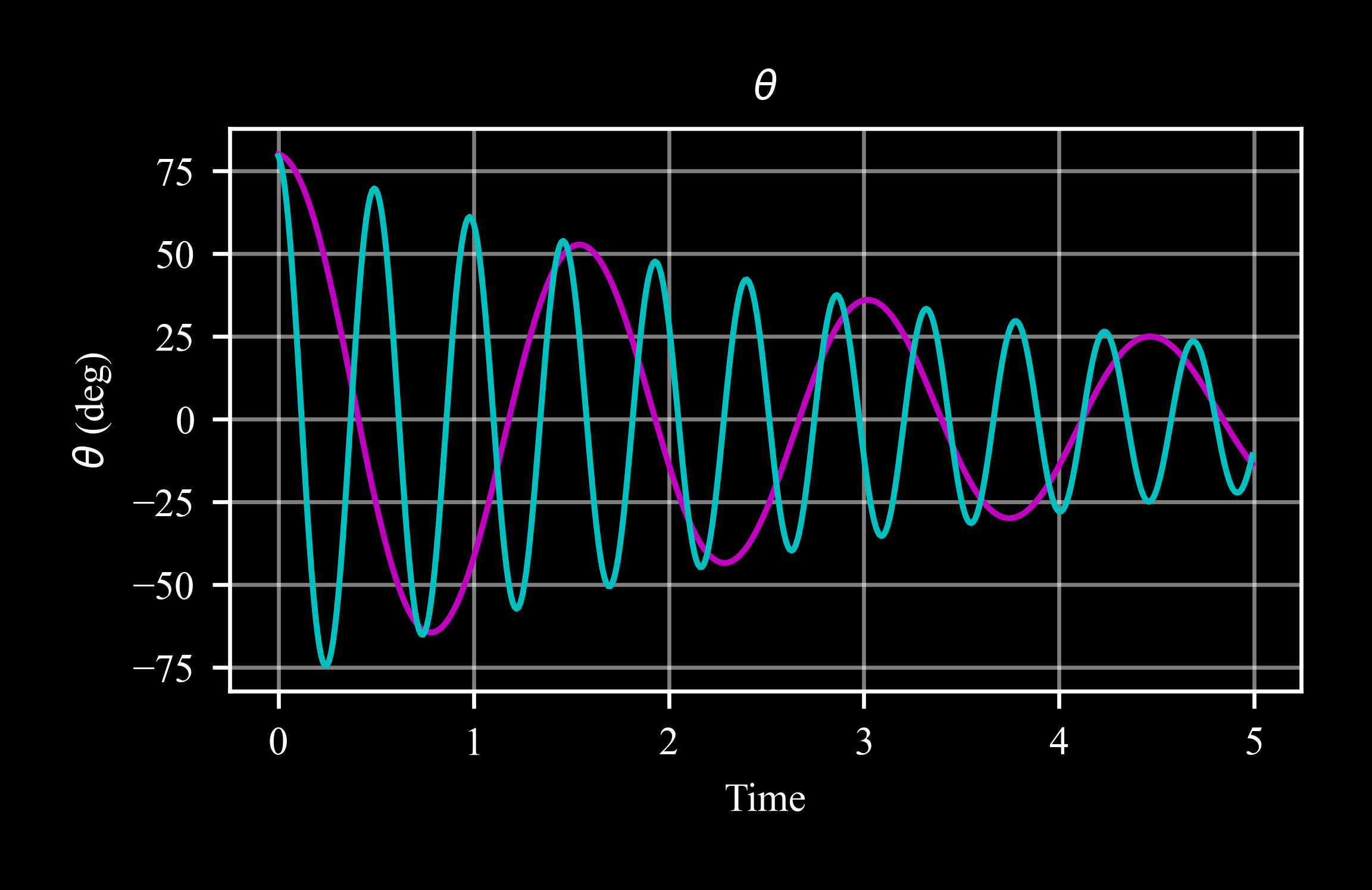
The moment of inertia determines how much torque is required for a desired angular acceleration about a rotational axis.

In this example, two physical pendulums with the same initial conditions show the effect of different moments of inertia on the time period of an oscillation:

\[T = 2 \cdot \pi \cdot \sqrt{{I \over m \cdot g \cdot l}}\]

where here \(m\) is the mass \(m = 1\), \(l\) is the length from the center of mass \(l = 1\), \(g\) is the gravity acceleration, and \(I\) is the moment of inertia about \(y\), \(I_{yy1} = 0.5, I_{yy2} = 0.05\)

Import required packages:

>>> import c4dynamics as c4d
>>> from matplotlib import pyplot as plt
>>> from scipy.integrate import odeint
>>> import numpy as np

Settings and initial condtions:

>>> b = 0.5
>>> dt = 0.01
>>> g = c4d.g_ms2
>>> theta0 = 80 * c4d.d2r
>>> rb05  = c4d.rigidbody(theta = theta0)
>>> rb05.I = [0, .5, 0]
>>> rb005 = c4d.rigidbody(theta = theta0)
>>> rb005.I = [0, .05, 0]

Physical pendulum dynamics:

>>> def pendulum(yin, t, Iyy):
...   theta, q = yin[7], yin[10]
...   yout = np.zeros(12)
...   yout[7] = q
...   yout[10] = -g * c4d.sin(theta) / Iyy - b * q
...   return yout

Main loop

>>> for ti in np.arange(0, 5, dt):
...   # Iyy = 0.5
...   rb05.X = odeint(pendulum, rb05.X, [ti, ti + dt], (rb05.I[1],))[1]
...   rb05.store(ti)
...   # Iyy = 0.05
...   rb005.X = odeint(pendulum, rb005.X, [ti, ti + dt], (rb005.I[1],))[1]
...   rb005.store(ti)

Plot results:

>>> rb05.plot('theta')
>>> rb005.plot('theta', ax = plt.gca(), color = 'c')
>>> plt.show()