Radar#
- class c4dynamics.sensors.radar.radar(origin=None, isideal=False, **kwargs)[source]#
Range-direction detector.
radar is a subclass of
seekerand utilizes its functionality and errors model for angular measurements. This documentation supplaments the information concerning range measurements. Refer toseekerfor the full documentation.The radar class models sensors that measure both the range and the direction to a target. The direction is measured in terms of azimuth and elevation. Sensors that provide precise range measurements typically use electro-magnetical technology, though other technologies may also be employed.
As a subclass of seeker, the radar can operate in one of two modes: ideal mode, providing precise range and direction measurements, or non-ideal mode, where measurements may be affected by errors such as scale factor, bias, and noise, according to the errors model. A random variable generation mechanism allows for Monte Carlo simulations.
- Parameters:
- Keyword Arguments:
rng_noise_std (float) – A standard deviation of the radar range. Default value for non-ideal radar: rng_noise_std = 1m.
bias_std (float) – The standard deviation of the bias error, [radians]. Defaults \(0.3°\).
scale_factor_std (float) – The standard deviation of the scale factor error, [dimensionless]. Defaults \(0.07 (= 7\%)\).
noise_std (float) – The standard deviation of the radar angular noise, [radians]. Default value for non-ideal radar: \(0.8°\).
dt (float) – The time-constant of the operational rate of the radar (below which the radar measures return None), [seconds]. Default value: \(dt = -1sec\) (no limit between calls to
measure).
Note the default values for angular parameters, bias_std, scale_factor_std, and noise_std, differ from those in a seeker object.
Functionality
At each sample the seeker returns measures based on the true geometry with the target.
Let the relative coordinates in an arbitrary frame of reference:
\[ \begin{align}\begin{aligned}dx = target.x - seeker.x\\dy = target.y - seeker.y\\dz = target.z - seeker.z\end{aligned}\end{align} \]The relative coordinates in the seeker body frame are given by:
\[x_b = [BR] \cdot [dx, dy, dz]^T\]where \([BR]\) is a Body from Reference DCM (Direction Cosine Matrix) formed by the seeker three Euler angles. See the rigidbody section below.
The azimuth and elevation measures are then the spatial angles:
\[ \begin{align}\begin{aligned}az = tan^{-1}{x_b[1] \over x_b[0]}\\el = tan^{-1}{x_b[2] \over \sqrt{x_b[0]^2 + x_b[1]^2}}\end{aligned}\end{align} \]Where:
\(az\) is the azimuth angle
\(el\) is the elevation angle
\(x_b\) is the target-radar position vector in radar body frame
For a radar object, the range is defined as:
\[range = \sqrt{x_b^2 + y_b^2 + z_b^2}\]Where:
\(range\) is the target-radar distance
\(x_b\) is the target-radar position vector in radar body frame

Fig-1: Range and angles definition#
Errors Model
The azimuth and elevation angles are subject to errors: scale factor, bias, and noise, as detailed in seeker. A radar instance has in addition range noise:
Range Noise: represents random variations or fluctuations in the measurements that are not systematic. The noise at each sample (measure) is a normally distributed variable with mean = 0 and std = rng_noise_std, where rng_noise_std is a radar parameter with default value of 1m.
Angular errors:
Bias: represents a constant offset or deviation from the true value in the seeker’s measurements. It is a systematic error that consistently affects the measured values. The bias of a seeker instance is a normally distributed variable with mean = 0 and std = bias_std, where bias_std is a parameter with default value of 0.3°.Scale Factor: a multiplier applied to the true value of a measurement. It represents a scaling error in the measurements made by the seeker. The scale factor of a seeker instance is a normally distributed variable with mean = 0 and std = scale_factor_std, , where scale_factor_std is a parameter with default value of 0.07.Noise: represents random variations or fluctuations in the measurements that are not systematic. The noise at each seeker sample (measure) is a normally distributed variable with mean = 0 and std = noise_std, where noise_std is a parameter with default value of 0.8°.
The errors model generates random variables for each radar instance, allowing for the simulation of different scenarios or variations in the radar behavior in a technique known as Monte Carlo. Monte Carlo simulations leverage this randomness to statistically analyze the impact of these biases and scale factors over a large number of iterations, providing insights into potential outcomes and system reliability.
Radar vs Seeker
The following table lists the main differences between
seekerandradarin terms of measurements and default error parameters:Angles
Range
\(σ_{Bias}\)
\(σ_{Scale Factor}\)
\(σ_{Angular Noise}\)
\(σ_{Range Noise}\)
Seeker
✔️
❌
\(0.1°\)
\(5%\)
\(0.4°\)
\(--\)
Radar
✔️
✔️
\(0.3°\)
\(7%\)
\(0.8°\)
\(1m\)
rigidbody
The radar class is also a subclass of
rigidbody, i.e. it suggests attributes of position and attitude and the manipulation of them.As a fundamental propety, the rigidbody’s state vector
Xsets the spatial coordinates of the radar:\[X = [x, y, z, v_x, v_y, v_z, {\varphi}, {\theta}, {\psi}, p, q, r]^T\]The first six coordinates determine the translational position and velocity of the radar while the last six determine its angular attitude in terms of Euler angles and the body rates.
Passing a rigidbody parameter as an origin sets the initial conditions of the radar.
Construction
A radar instance is created by making a direct call to the radar constructor:
>>> rdr = c4d.sensors.radar()
Initialization of the instance does not require any mandatory arguments, but the radar parameters can be determined using the **kwargs argument as detailed above.
Examples
Import required packages:
>>> import c4dynamics as c4d
>>> from matplotlib import pyplot as plt
>>> import numpy as np
Target
For the examples below let’s generate the trajectory of a target with constant velocity:
>>> tgt = c4d.datapoint(x = 1000, y = 0, vx = -80 * c4d.kmh2ms, vy = 10 * c4d.kmh2ms)
>>> for t in np.arange(0, 60, 0.01):
...   tgt.inteqm(np.zeros(3), .01)
...   tgt.store(t)
The method
inteqmof thedatapointclass integrates the 3 degrees of freedom equations of motion with respect to the input force vector (np.zeros(3) here).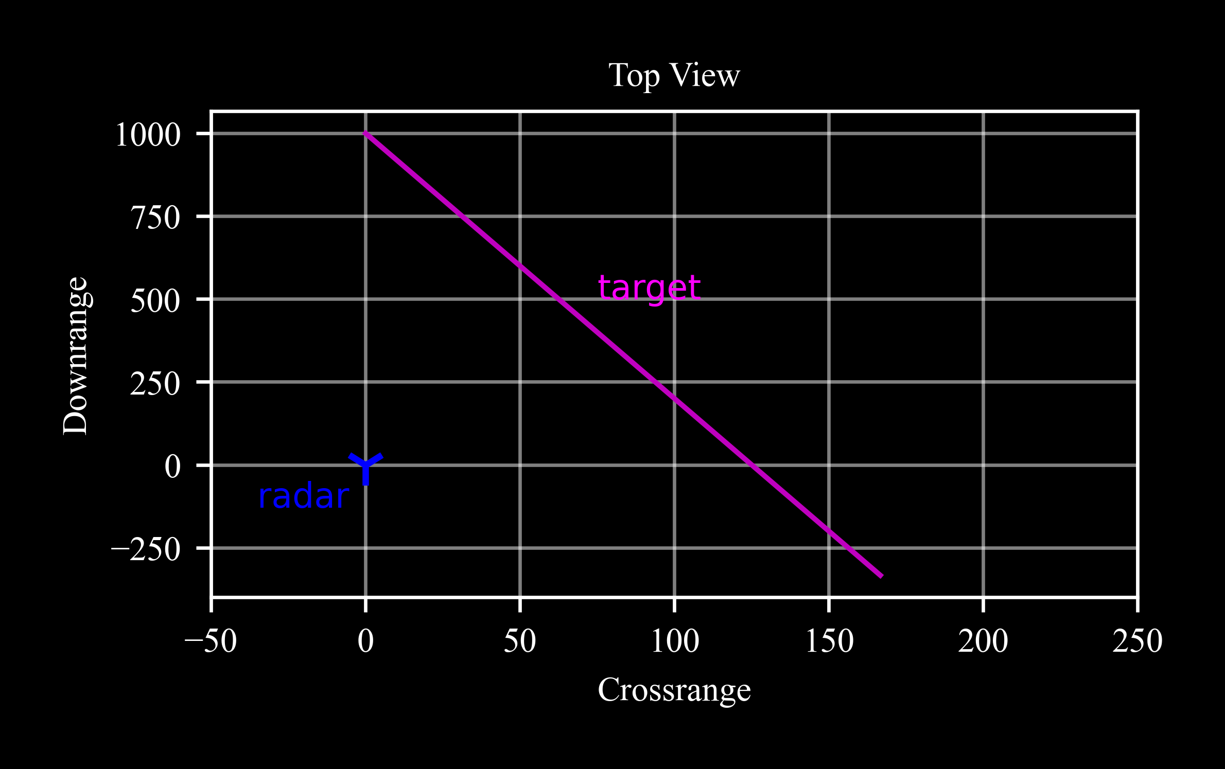
Since the call to
measurerequires a target as a datapoint object we utilize a custom create function that returns a new datapoint object for a given X state vector in time.c4d.kmh2msconverts kilometers per hour to meters per second.c4d.r2dconverts radians to degrees.c4d.d2rconverts degrees to radians.
Origin
Let’s also introduce a pedestal as an origin for the radar. The pedestal is a rigidbody object with position and attitude:
>>> pedestal = c4d.rigidbody(z = 30, theta = -1 * c4d.d2r)
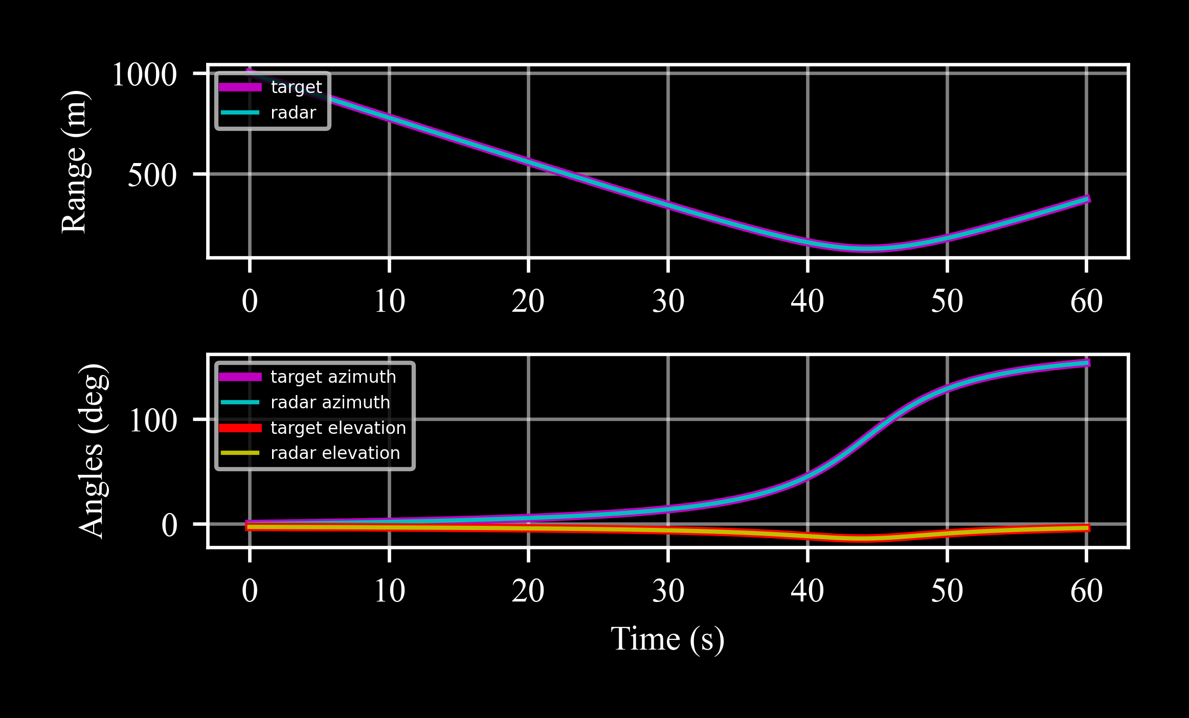
Ideal Radar
Measure the target position with an ideal radar:
>>> rdr_ideal = c4d.sensors.radar(origin = pedestal, isideal = True)
>>> for x in tgt.data():
...   rdr_ideal.measure(c4d.create(x[1:]), t = x[0], store = True)
Comparing the radar measurements with the true target angles requires converting the relative position to the radar body frame:
>>> dx =  tgt.data('x')[1] - rdr_ideal.x
>>> dy =  tgt.data('y')[1] - rdr_ideal.y
>>> dz =  tgt.data('z')[1] - rdr_ideal.z
>>> Xb = np.array([rdr_ideal.BR @ [X[1] - rdr_ideal.x, X[2] - rdr_ideal.y, X[3] - rdr_ideal.z] for X in tgt.data()])
where
rdr_ideal.BRis a Body from Reference DCM (Direction Cosine Matrix) formed by the radar three Euler anglesNow az_true and el_true are the true target angles with respect to the radar, and rng_true is the true range (atan2d is an aliasing of numpy’s arctan2 with a modification returning the angles in degrees):
>>> az_true = c4d.atan2d(Xb[:, 1], Xb[:, 0])
>>> el_true = c4d.atan2d(Xb[:, 2], c4d.sqrt(Xb[:, 0]**2 + Xb[:, 1]**2))
>>> # plot results
>>> fig, axs = plt.subplots(2, 1)
>>> # range
>>> axs[0].plot(tgt.data('t'), c4d.norm(Xb, axis = 1), label = 'target')
>>> axs[0].plot(*rdr_ideal.data('range'), label = 'radar')
>>> # angles
>>> axs[1].plot(tgt.data('t'), c4d.atan2d(Xb[:, 1], Xb[:, 0]), label = 'target azimuth')
>>> axs[1].plot(*rdr_ideal.data('az', scale = c4d.r2d), label = 'radar azimuth')
>>> axs[1].plot(tgt.data('t'), c4d.atan2d(Xb[:, 2], c4d.sqrt(Xb[:, 0]**2 + Xb[:, 1]**2)), label = 'target elevation')
>>> axs[1].plot(*rdr_ideal.data('el', scale = c4d.r2d), label = 'radar elevation')
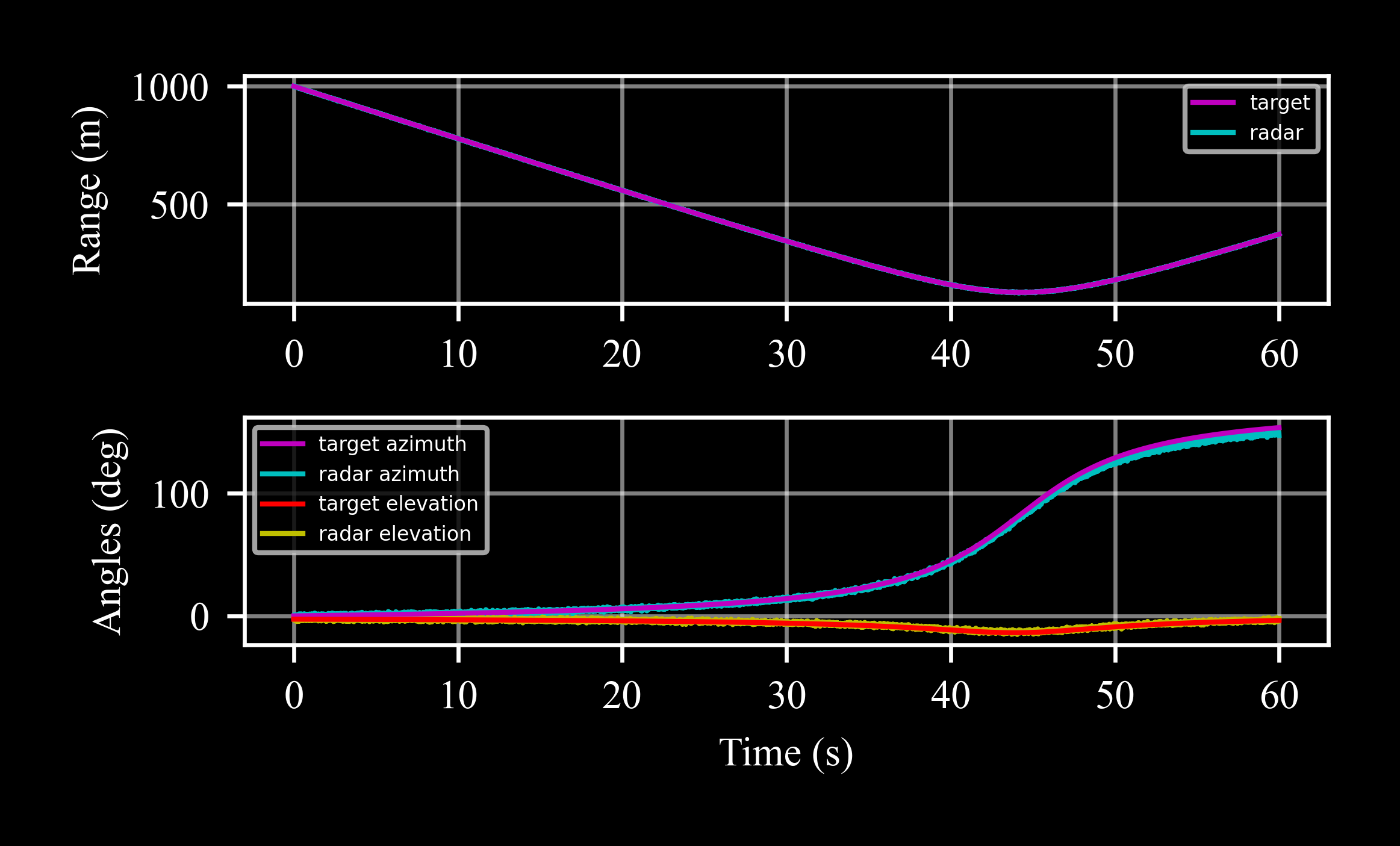
Non-ideal Radar
Measure the target position with a non-ideal radar. The radar’s errors model introduces bias, scale factor, and noise that corrupt the measurements:
To reproduce the result, let’s set the random generator seed (61 is arbitrary):
>>> np.random.seed(61)
>>> rdr = c4d.sensors.radar(origin = pedestal)
>>> for x in tgt.data():
...   rdr.measure(c4d.create(x[1:]), t = x[0], store = True)
Results with respect to an ideal radar:
>>> fig, axs = plt.subplots(2, 1)
>>> # range
>>> axs[0].plot(*rdr_ideal.data('range'), label = 'target')
>>> axs[0].plot(*rdr.data('range'), label = 'radar')
>>> # angles
>>> axs[1].plot(*rdr_ideal.data('az', scale = c4d.r2d), label = 'target azimuth')
>>> axs[1].plot(*rdr.data('az', scale = c4d.r2d), label = 'radar azimuth')
>>> axs[1].plot(*rdr_ideal.data('el', scale = c4d.r2d), label = 'target elevation')
>>> axs[1].plot(*rdr.data('el', scale = c4d.r2d), label = 'radar elevation')
target labels mean the true position as measured by an ideal radar.
The bias, scale factor, and noise that used to generate these measures can be examined by:
>>> rdr.rng_noise_std
1.0
>>> rdr.bias * c4d.r2d
0.13...
>>> rdr.scale_factor
0.96...
>>> rdr.noise_std * c4d.r2d
0.8
Points to consider here:
The scale factor error increases with the angle, such that for a \(7%\) scale factor, the error of \(Azimuth = 100°\) is \(7°\), whereas the error for \(Elevation = -15°\) is only \(-1.05°\).
The standard deviation of the noise in the two angle channels is the same. However, as the Elevation values are confined to a smaller range, the effect appears more pronounced there.
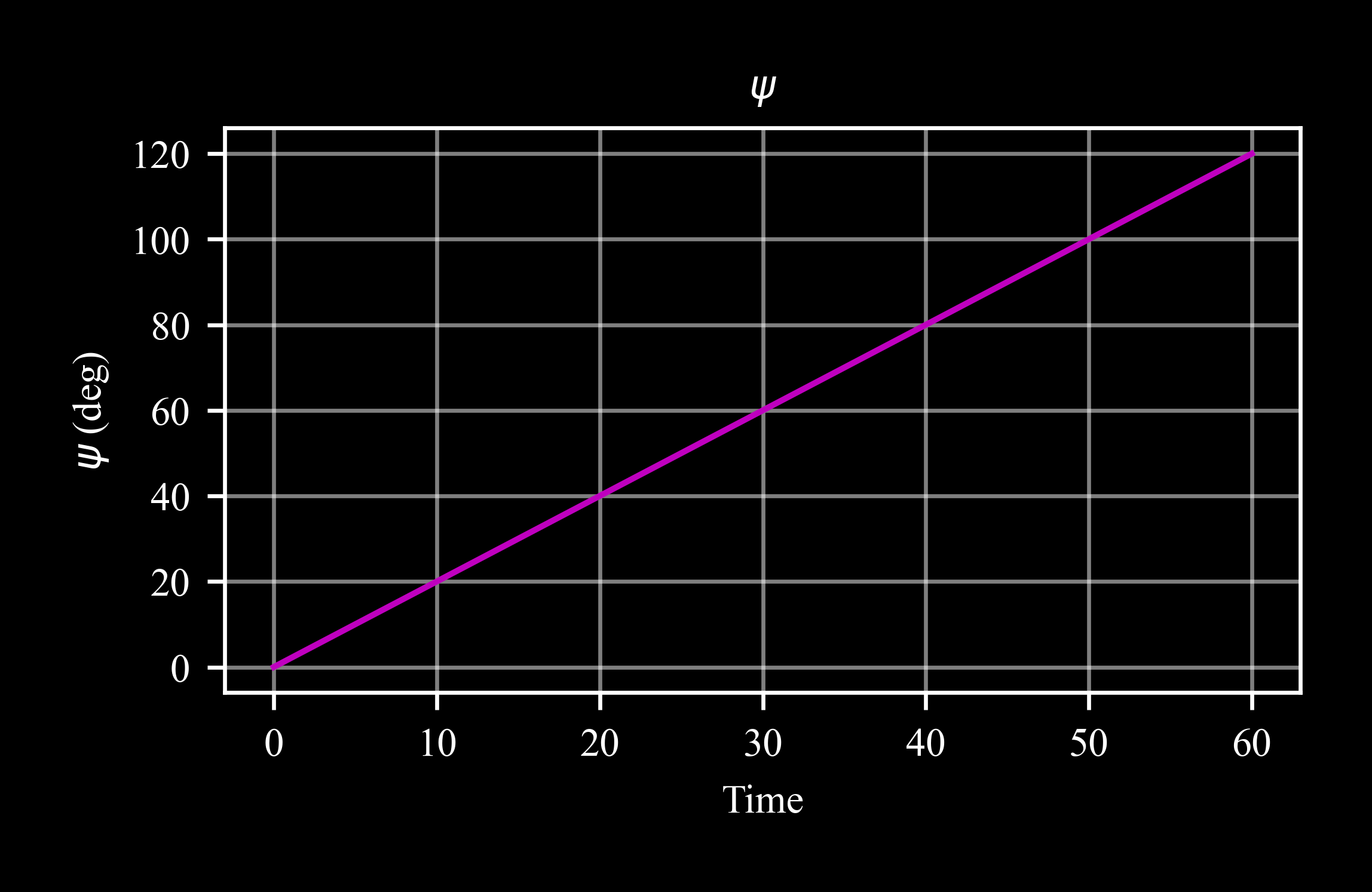
Rotating Radar
Measure the target position with a rotating radar. The radar origin is yawing (performed by the increment of \(\psi\)) in the direction of the target motion:
>>> rdr = c4d.sensors.radar(origin = pedestal)
>>> for x in tgt.data():
...   rdr.psi += .02 * c4d.d2r
...   rdr.measure(c4d.create(x[1:]), t = x[0], store = True)
...   rdr.store(x[0])
The radar yaw angle:
And the target angles with respect to the yawing radar are:
>>> fig, axs = plt.subplots(2, 1)
>>> # range
>>> axs[0].plot(*rdr_ideal.data('range'), label = 'ideal static')
>>> axs[0].plot(*rdr.data('range'),label = 'non-ideal yawing')
>>> # angles
>>> axs[1].plot(*rdr_ideal.data('az', c4d.r2d), label = 'az: ideal static')
>>> axs[1].plot(*rdr.data('az', c4d.r2d), label = 'az: non-ideal yawing')
>>> axs[1].plot(*rdr_ideal.data('el', scale = c4d.r2d), label = 'el: ideal static')
>>> axs[1].plot(*rdr.data('el', scale = c4d.r2d), label = 'el: non-ideal yawing')
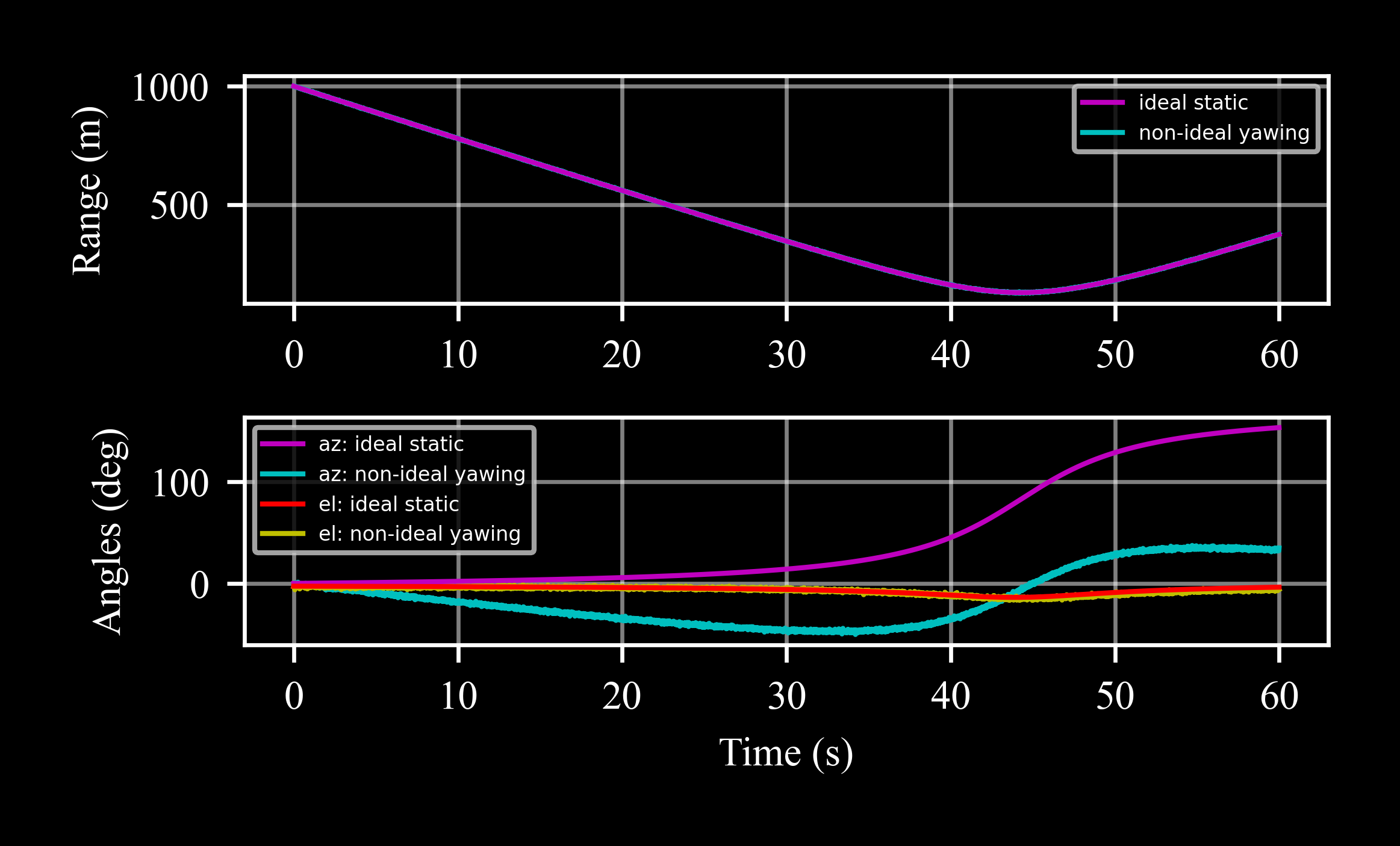
The rotation of the radar with the target direction keeps the azimuth angle limited, such that non-rotating radars with limited FOV (field of view) would have lost the target.
Operation Time
By default, the radar returns measurments for each call to
measure. However, setting the parameter dt to a positive number makes measure return None for any t < last_t + dt, where t is the current measure time, last_t is the last measurement time, and dt is the radar time-constant:>>> np.random.seed(770) >>> tgt = c4d.datapoint(x = 100, y = 100) >>> rdr = c4d.sensors.radar(dt = 0.01) >>> for t in np.arange(0, .025, .005): ... print(f'{t}: {rdr.measure(tgt, t = t)}') 0.0: (0.7..., 0.01..., 140.1...) 0.005: (None, None, None) 0.01: (0.72..., -0.04..., 142.1...) 0.015: (None, None, None) 0.02: (0.72..., -0.003..., 140.4...)
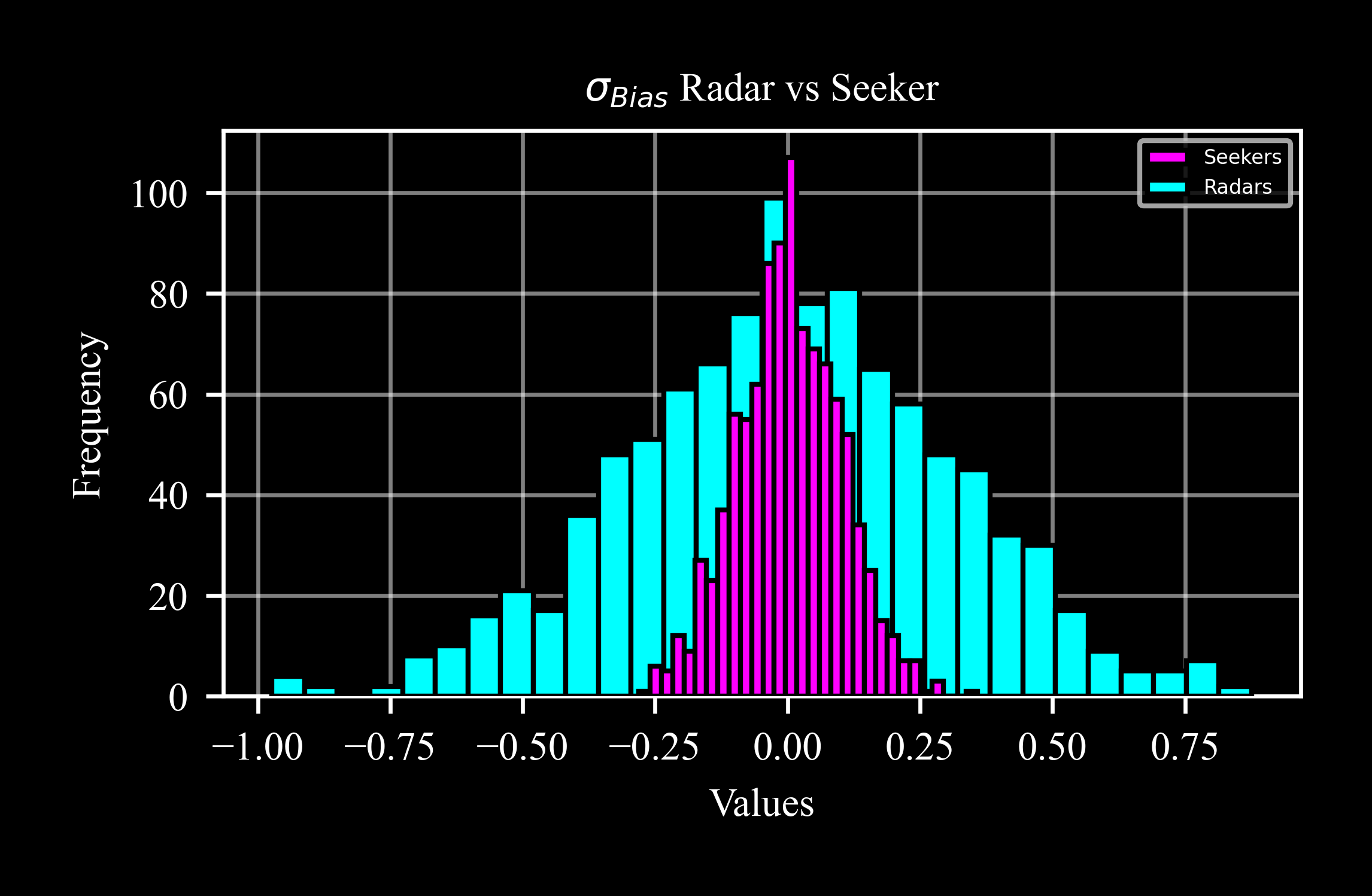
Random Distribution
The distribution of normally generated random variables is characterized by its bell-shaped curve, which is symmetric about the mean. The area under the curve represents probability, with about 68% of the data falling within one standard deviation (1σ) of the mean, 95% within two, and 99.7% within three, making it a useful tool for understanding and predicting data behavior.
In radar objects, and seeker objects in general, the bias and scale factor vary among different instances to allow a realistic simulation of performance behavior in a technique known as Monte Carlo.
Let’s examine the bias distribution across
mutliple radar instances with a default bias_std = 0.3° in comparison to seeker instances with a default bias_std = 0.1°:
>>> from c4dynamics.sensors import seeker, radar
>>> seekers = []
>>> radars = []
>>> for i in range(1000):
...   seekers.append(seeker().bias * c4d.r2d)
...   radars.append(radar().bias * c4d.r2d)
The histogram highlights the broadening of the distribution as the standard deviation increases:
>>> ax = plt.subplot()
>>> ax.hist(seekers, 30, label = 'Seekers')
>>> ax.hist(radars, 30, label = 'Radars')
Properties
Gets and sets the object's bias.
Gets and sets the object's scale_factor.
Methods
radar.measure(target[, t, store])Measures range, azimuth and elevation between the radar and a target.