c4dynamics.states.state.state.plot

state.plot(var, scale=1, ax=None, filename=None, darkmode=True, **kwargs)

Draws plots of variable evolution over time.

This method plots the evolution of a state variable over time. The resulting plot can be saved to a directory if specified.

Parameters:

• var (str) – The name of the variable or parameter to be plotted.

• scale (float or int, optional) – A scaling factor to apply to the variable values. Defaults to 1.

• ax (matplotlib.axes.Axes, optional) – An existing Matplotlib axis to plot on. If None, a new figure and axis will be created, by default None.

• filename (str, optional) – Full file name to save the plot image. If None, the plot will not be saved, by default None.

• darkmode (bool, optional) – Directory path to save the plot image. If None, the plot will not be saved, by default None.

• **kwargs (dict, optional) – Additional key-value arguments passed to matplotlib.pyplot.plot. These can include any keyword arguments accepted by plot, such as color, linestyle, marker, etc.

Returns:

ax (matplotlib.axes.Axes.) – Matplotlib axis of the derived plot.

Note

• The default color is set to ‘m’ (magenta).

• The default linewidth is set to 1.2.

Examples

Import required packages:

>>> import c4dynamics as c4d
>>> from matplotlib import pyplot as plt
>>> import numpy as np

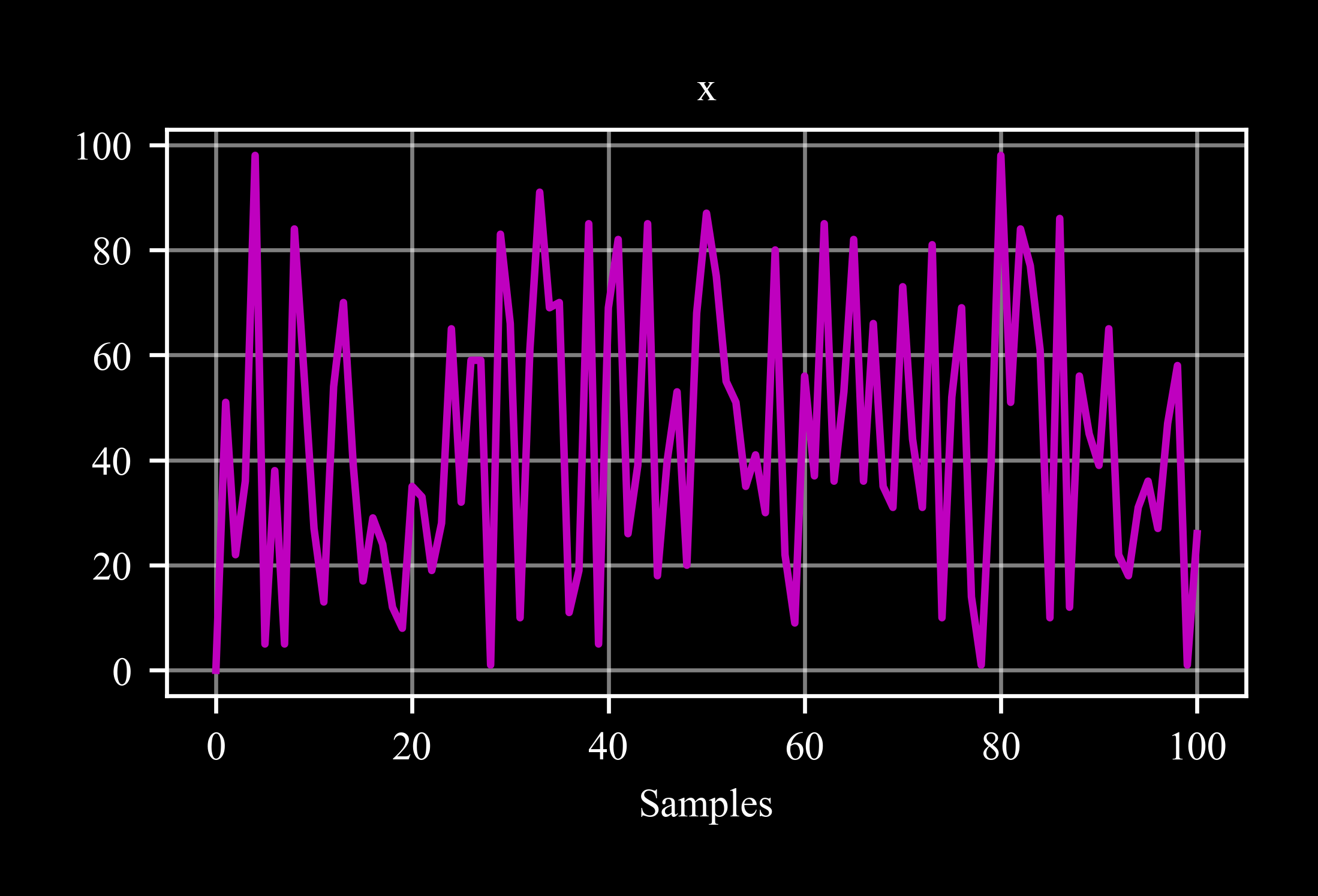
Plot an arbitrary state variable and save:

>>> s = c4d.state(x = 0, y = 0)
>>> s.store()
>>> for _ in range(100):
...   s.x = np.random.randint(0, 100, 1)
...   s.store()
>>> s.plot('x', filename = 'x.png')   
>>> plt.show()

Interactive mode:

>>> plt.switch_backend('TkAgg')
>>> s.plot('x')   
>>> plt.show(block = True)

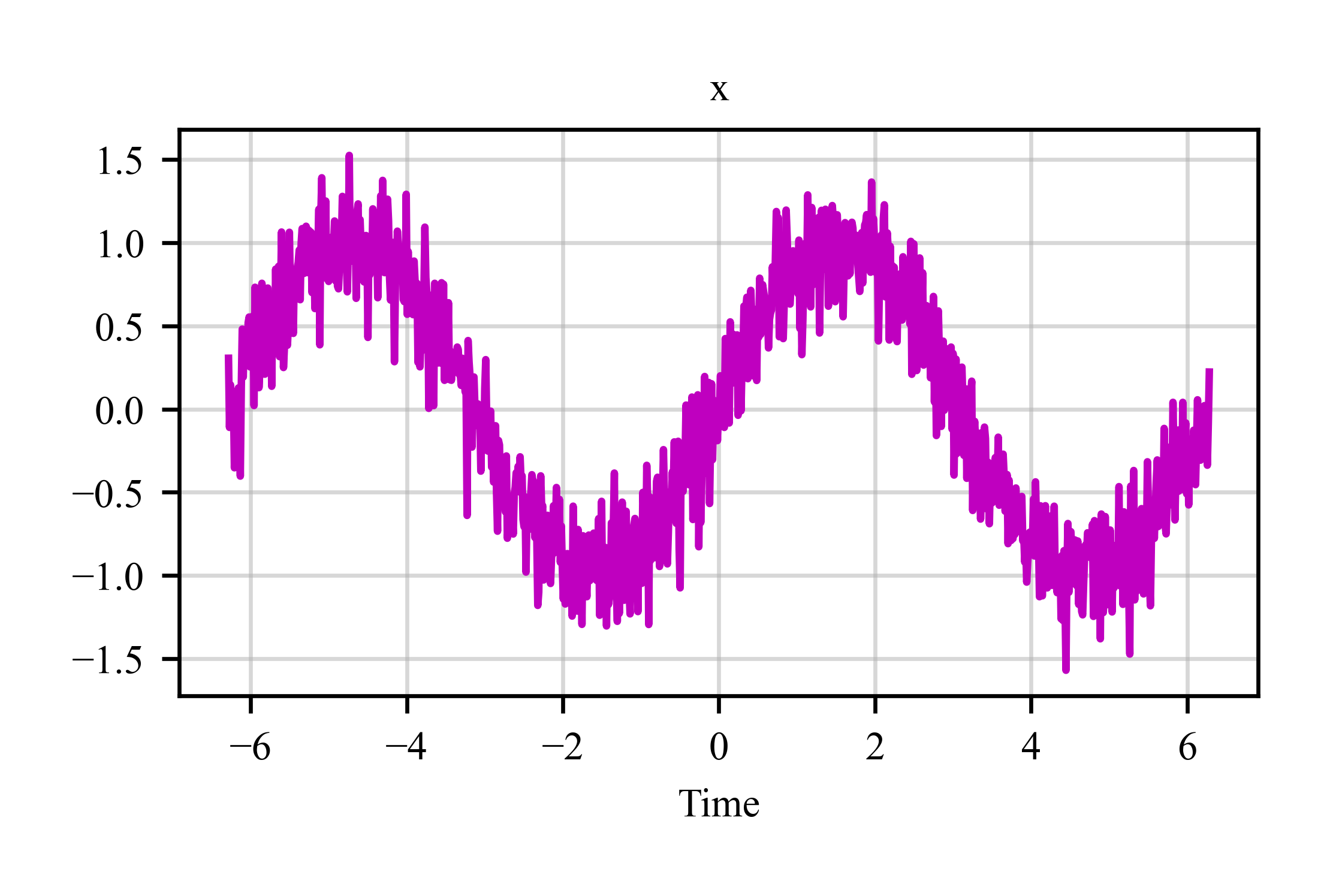
Dark mode off:

>>> s = c4d.state(x = 0)
>>> s.xstd = 0.2
>>> for t in np.linspace(-2 * c4d.pi, 2 * c4d.pi, 1000):
...   s.x = c4d.sin(t) + np.random.randn() * s.xstd
...   s.store(t)
>>> s.plot('x', darkmode = False)    
>>> plt.show()

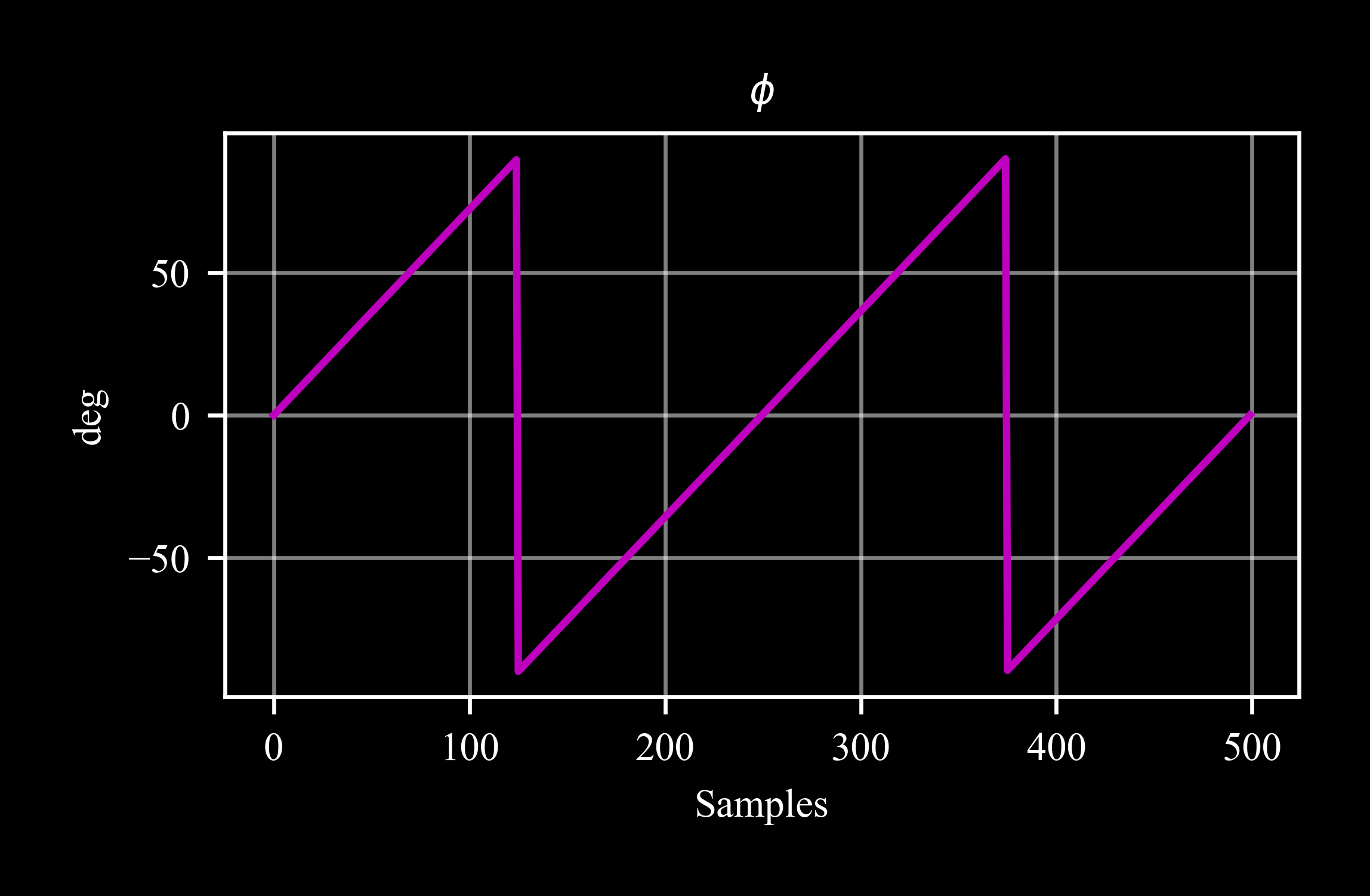
Scale plot:

>>> s = c4d.state(phi = 0)
>>> for y in c4d.tan(np.linspace(-c4d.pi, c4d.pi, 500)):
...   s.phi = c4d.atan(y)
...   s.store()
>>> s.plot('phi', scale = c4d.r2d)  
>>> plt.gca().set_ylabel('deg') 
>>> plt.show()

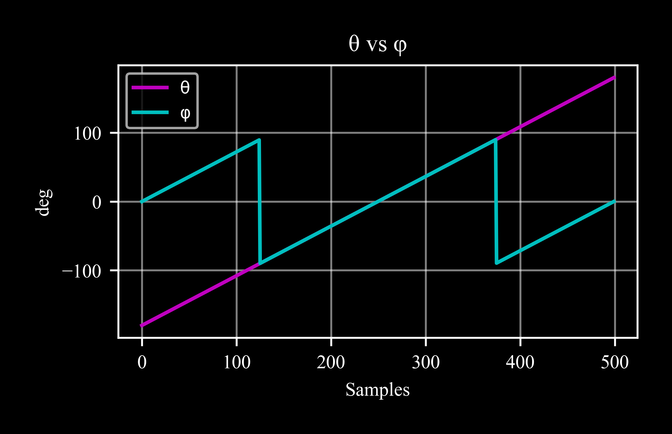
Given axis:

>>> plt.subplots(1, 1)  
>>> plt.plot(np.linspace(-c4d.pi, c4d.pi, 500) * c4d.r2d, 'm')   
>>> s.plot('phi', scale = c4d.r2d, ax = plt.gca(), color = 'c')    
>>> plt.gca().set_ylabel('deg')  
>>> plt.legend(['θ', 'φ'])  
>>> plt.show()

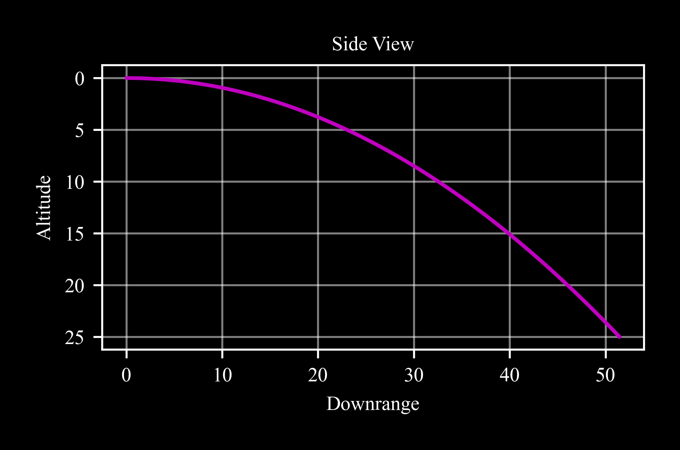
Top view + side view - options of datapoint and rigidbody objects:

>>> dt = 0.01
>>> floating_balloon = c4d.datapoint(vx = 10 * c4d.k2ms)
>>> floating_balloon.mass = 0.1
>>> for t in np.arange(0, 10, dt):
...   floating_balloon.inteqm(forces = [0, 0, .05], dt = dt)   
...   floating_balloon.store(t)
>>> floating_balloon.plot('side')
>>> plt.gca().invert_yaxis()
>>> plt.show()