To download this notebook, click the download icon in the toolbar above and select the .ipynb format.
For any questions or comments, please open an issue on the c4dynamics issues page.
Proportional Navigation Guidance - 6 Degrees of Freedom Simulation#
Six Degrees Of Freedom (6DOF) simulation of a guided aircraft, modeling its dynamics, aerodynamics, and control system.
Contents#
Introduction
Simulation Overview
Setup and Initial Conditions
Main Loop
Miss Distance
Results
Summary
1. Introduction#
This notebook presents a six degrees of freedom (6DOF) simulation of a guided aircraft, capturing the dynamics, aerodynamics, control system, and seeker behavior. The guided aircraft in this case is a missile pursuing a target using a proportional navigation guidance law. The simulation includes both translational and rotational dynamics, accounts for aerodynamic forces, and models control surface deflections in response to seeker feedback.
By walking through the setup, implementation, and results, the notebook provides a complete view of how 6DOF guidance algorithms operate in practice. The missile, target, and seeker are modeled using the c4dynamics — an open-source framework for algorithm engineering that provides state objects to represent dynamic entities in space and time. The details of the missile model and the guidance system are based on the example in Chapter 12 of the Military Handbook of Missile Flight Simulation [1].
2. Simulation Overview#
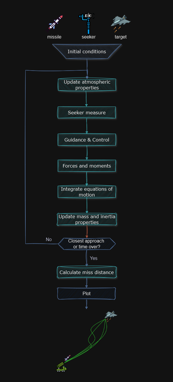
Figure 1: Simulation OverviewThe simulation then enters a main loop, which iterates at a time step of 5 milliseconds until termination conditions are met. Each iteration involves the following steps:
Update Atmospheric Properties: Atmospheric conditions, including pressure, density, and speed of sound, are calculated based on the missile’s current altitude using an atmospheric model. These properties determine aerodynamic forces and the Mach number, influencing the missile’s behavior.
Seeker Measurement: The line-of-sight seeker tracks angular rate variations between the missile and the target, providing critical data for trajectory adjustments. This step ensures the missile can track the target’s relative position and velocity.
Guidance & Control: After a 0.5-second delay to allow the missile to gain sufficient speed, the guidance system activates. It uses the seeker’s measurements to generate control commands, adjusting the missile’s pitch and yaw through control surface deflections to align its trajectory with the target.
Forces & Moments: Forces acting on the missile, including aerodynamic (lift, drag, axial, and normal), propulsion (thrust), and gravity, are computed. Aerodynamic moments (pitch and yaw) are also calculated based on the missile’s orientation and Mach number. These forces and moments are transformed into the inertial frame using the missile’s rotation matrix.
Integrate Equations of Motion: The missile’s translational and rotational equations of motion are integrated using a numerical method to update its position, velocity, Euler angles, and angular rates. The target’s position is similarly updated if it is moving, assuming no external forces for a non-maneuvering target.
Update Mass and Inertia Properties: As the missile consumes fuel, its mass and inertia properties are updated to reflect changes in dynamics.
After each iteration, the simulation evaluates termination conditions. If the range rate changes sign (indicating the closest approach), the missile’s altitude drops below zero, or the simulation time exceeds 100 seconds, the loop exits. Otherwise, it returns to updating atmospheric properties for the next iteration.
Upon termination, the simulation calculates the miss distance, determining the minimum distance between the missile and the target at the point of closest approach. This is approximated by analyzing the relative position vector perpendicular to the flight path and estimating the time of closest approach.
Finally, the results are shown: Trajectory Plots, Euler Angles, and Line-of-Sight Rates. These plots provide insights into the missile’s dynamic behavior and the guidance system’s performance.
The program utilizes the following components of c4dynamics:
Object |
Module |
Description |
|---|---|---|
missile |
The missile is modeled as a rigid body, representing a mass in space with defined length and orientation |
|
target |
The target is represented as a datapoint object, modeling a point mass in space |
|
seeker |
line-of-sight seeker |
|
g_ms2 |
Gravity constant in meters per second |
|
r2d |
Radians to degrees conversion constant |
|
plotdefaults |
Setting default properties on a matplotlib axis |
In addition, some operations use c4dynamics modules explicitly. Among them:
missile.RB uses the rotmat module to rotate a vector from the body frame (B) to a reference frame (R).
missile.inteqm() intgrates the equations of motion for a given vector of forces.
Let’s start.
3. Setup and Initial Conditions#
Import packages#
[20]:
import c4dynamics as c4d
import numpy as np
[21]:
from dof6_modules import control_system, engine, aerodynamics
Times setup#
[22]:
t  = 0
tf = 100
dt = 5e-3
Target#
datapoint object which means it has all the attributes of a mass in space:Position: target.x, target.y, target.z.Velocity: target.vx, target.vy, target.vz.It also has mass: target.mass (necessary for solving the equations of motion in the case of accelerating motion)
In this example, the target is initialized with specific positions along the three axes and a velocity component only along the x-axis.
[23]:
target = c4d.datapoint(x = 4000, y = 1000, z = -3000, vx = -250)
Missile#
rigidbody object, i.e. it has all the attributes of a datapoint, but also includes:Body (Euler) angles: missile.phi, missile.theta, missile.psi.Angular rates: missile.p, missile.q, missile.r (rotation about \(x\), \(y\), and \(z\), respectively).Since the rocket engine operates through fuel combustion, the missile’s mass properties vary over time.
To enable mass recalculations during runtime, it is advisable to store the missile’s initial conditions.
As \(i_{yy}\) and \(i_{zz}\) are equal here it’s enough to save just one of them. However, the initial position and initial attitude of any object (datapoint, rigidbody) are always saved on instantiation.
The dimensions here are SI (i.e. seconds, meters, kilograms).
[24]:
m0      = 85        # initial mass, kg
mbo     = 57        # burnout mass, kg
iyy0    = 61        # initial momoent of inertia about y and z
ibo     = 47        # iyy izz at burnout
xcm0    = 1.55      # initial distance from nose to center of mass, m
xcmbo   = 1.35      # distance from nose to center of mass after burnout, m
[25]:
missile = c4d.rigidbody()
[26]:
missile.mass = m0
missile.I = [0, iyy0, iyy0]
missile.xcm = xcm0
Modules#
[27]:
seeker = c4d.sensors.lineofsight(dt, tau1 = 0.01, tau2 = 0.01)
ctrl   = control_system(dt)
eng    = engine()
aero   = aerodynamics()
Initial conditions#
The initial missile direction is calculated by employing a simple algorithm in which the missile is pointed \(30°\) below the line-of-sight to the target at the instant of launch. The missile angular rates at launch are assumed to be negligible.
[28]:
rTM           = target.Position - missile.Position
rTMnorm       = np.linalg.norm(rTM)
ucl           = rTM / rTMnorm # center line unit vector

pitch_tgt   = np.arctan(ucl[2] / np.linalg.norm(ucl[:2])) * c4d.r2d
heading     = 30 # +30 tilts head down since z positive is downward.
pitch_lnch  = pitch_tgt + heading
ucl[2]      = np.linalg.norm(ucl[:2]) * np.tan(pitch_lnch * c4d.d2r)
ucl         = ucl / np.linalg.norm(ucl)

missile.vx, missile.vy, missile.vz = 30 * ucl # 30m/s is the missile initial velocity
missile.psi   = np.arctan(ucl[1] / ucl[0])
missile.theta = np.arctan(-ucl[2] / np.sqrt(ucl[0]**2 + ucl[1]**2))
missile.phi   = 0.
u, v, w       = missile.BR @ missile.Velocity
vc            = np.zeros(3)
ab_cmd        = np.zeros(3)
h             = -missile.z # missile altitude above sea level

alpha       = 0
beta        = 0
alpha_total = 0
d_pitch     = 0
d_yaw       = 0

delta_data   = []
omegaf_data  = []
acc_data     = []
aoa_data     = []
moments_data = []
Frame of coordinates and DCM#
The property missile.BR returns a Body from Inertial DCM (Direction Cosine Matrix) in 3-2-1 order. Using this matrix, the missile velocity vector in the inertial frame of coordinates is rotated to represent the velocity in the body frame of coordinates.
The inertial frame is determined by the frame that the initial Euler angles refer to. In this example, the reference of the Euler angles are as follows:
\(\varphi\): rotation about \(x\)
\(\theta\): rotation about \(y\)
\(\psi\): rotation about \(z\)
The frame axes convention is given by:
\(x\): parallel to flat earth in the direction of the missile centerline
\(y\): completes a right-hand system
\(z\): positive downward
4. Main loop#
The main simulation loop performs the following steps:
Geometry
Update the target and the missile position and attitude according to the kinematics and initial conditions.
Estimate the line-of-sight angular rate between the missile and target. Guidance law
Compute the proportional navigation command
Generate wing deflection commands for the missile. Kinematic equations
Calculate forces and moments acting on the missile.
Integrate the missile’s equations of motion.
Integrate the target’s equations of motion.
Here’s a thorough explanation of each block:
Geometry#
The target and missile positions are set by initial conditions or updated via kinematic differential equations.
Then, the missile’s seeker measures the line-of-sight (LOS) vector, approximated as \(r_{TM}\), and provides angular rates to the guidance system. The seeker resolves the LOS unit vector \(u_R = r_{TM}/|r_{TM}|\) and computes the LOS angular rate as:
where:
\(r_{TM} = r_T - r_M\) is the relative position vector (target minus missile),
\(v_{TM} = v_T - v_M\) is the relative velocity.
The geometry is further characterized by the range \(R = |r_{TM}|\) and the closing velocity \(V_c = -u_R \cdot v_{TM}\), which determines the rate of approach.
Guidance Law#
The guidance law employs proportional navigation (PN), which aligns the missile’s velocity vector with the LOS to the target for interception.
PN uses the LOS angular rate to generate corrective acceleration commands. The core equation is:
where:
\(a_c\) is the acceleration command (perpendicular to the missile’s velocity)
\(N\) is the navigation gain (typically \(3–5\), here: \(4\))
\(V_m\) is the missile’s speed
\(\omega\) is the LOS angular rate vector
\(u_R\) is the unit vector along the LOS.
The LOS angular rate is measured by the seeker and calculated as described in the Geometry section.
PN aims to nullify the LOS rate \((\omega → 0)\) to ensure a collision course. The commanded acceleration is transformed into the missile’s body frame using the rotation matrix (derived from Euler angles) and implemented via control surface deflections (e.g., pitch and yaw fins).
Kinematic Differential Equations#
The kinematic differential equations govern the missile’s motion in a six degrees of freedom (6DOF) simulation, capturing both translational and rotational dynamics. These equations describe how the missile’s position, velocity, and attitude evolve under forces (e.g., aerodynamic, propulsion, gravity) and moments.
The target is treated as a point mass (with no attitude) and resolved in three degrees of freedom with no forces exerted.
For translational motion, Newton’s second law is applied in the inertial frame:
where:
\(v = [v_x, v_y, v_z]\) is the velocity vector
\(F\) is the total force vector
\(m\) is the missile’s mass.
Position is updated via
where:
\(r = [x, y, z]\).
For rotational motion, the attitude is represented by Euler angles \((\varphi, \theta, \psi)\) — roll, pitch, and yaw, respectively.
The Euler angle derivatives relate the body angular rates \((p, q, r)\) to the attitude rates:
These equations account for the missile’s orientation, updated numerically to reflect changes due to aerodynamic moments and control surface deflections.
The moments follow Euler’s equations for a rigid body:
where:
\(\omega = [p, q, r]\)
\(I\) is the inertia tensor
\(M\) is the moment vector.
This framework ensures accurate propagation of the missile’s dynamic state.
eqm module of c4dynamics and is encapsulated in the lines:missile.inteqm()target.inteqm()The target, as a datapoint, runs the int3 method which integrates the translational equations as given. The missile, as a rigidbody object, runs int6 and integrates the translation and rotational equations as given by eqm6. For a detailed explanation of the integration and differential equations, see the introduction to the equations of motion solvers module.
The simulation runs until one of the following conditions is satisfied:
The range rate changes sign
The missile hits the ground
The simulation time is over
Comments are introduced inline.
[29]:
while t <= tf and h >= 0 and vc[0] >= 0:

    # relative position
    vTM = target.Velocity - missile.Velocity # missile-target relative velocity
    rTM = target.Position - missile.Position # relative position

    # relative velcoity
    rTMnorm = np.linalg.norm(rTM) # for next round
    uR     = rTM / rTMnorm # unit range vector
    vc     = -uR * vTM # closing velocity

    # calculate the line-of-sight rates
    wf = seeker.measure(rTM, vTM)
    omegaf_data.append([wf[1], wf[2]])

    # atmospheric calculations
    pressure, rho, vs = aerodynamics.alt2atmo(h)

    mach = missile.V() / vs # mach number
    Q = 1 / 2 * rho * missile.V()**2 # dynamic pressure


    # guidance and control
    if t >= 0.5:
        '''
        The guidance is initiated half a second after launch in
        order to permit the missile to gain enough speed so that
        it can be controlled.
        Then the line-of-sight rate vector and the missile velocity
        are used to base maneuver commands and the control system
        responds by deflecting the control surfaces.
        '''
        Gs       = 4 * missile.V()
        a_cmd     = Gs * np.cross(wf, ucl)
        ab_cmd   = missile.BR @ a_cmd
        afp, afy = ctrl.update(ab_cmd, Q)
        d_pitch  = afp - alpha
        d_yaw    = afy - beta

    acc_data.append(ab_cmd)
    delta_data.append([d_pitch, d_yaw])


    ''' forces and moments '''

    # aerodynamic forces
    cL, cD = aero.f_coef(mach, alpha_total) # get lift and drag coefficients based on Mach number and angle of attack
    L = Q * aero.s * cL     # compute lift force using dynamic pressure, reference area, and lift coefficient
    D = Q * aero.s * cD     # compute drag force using dynamic pressure, reference area, and drag coefficient


    # aero axial force
    A = D * np.cos(alpha_total) - L * np.sin(alpha_total)
    # aero normal force
    N = D * np.sin(alpha_total) + L * np.cos(alpha_total)

    # convert aerodynamic forces to body frame coordinates
    fAb = np.array([ -A     # axial force in body X-direction (negative because drag acts against velocity)
                    , N * (-v / np.sqrt(v**2 + w**2))   # normal force component in body Y-direction
                    , N * (-w / np.sqrt(v**2 + w**2))]) # normal force component in body Z-direction
    fAe = missile.RB @ fAb  # rotate aerodynamic forces to inertial frame

    # aerodynamic moments
    cM, cN = aero.m_coef(mach, alpha, beta, d_pitch, d_yaw
                        , missile.xcm, Q, missile.V(), fAb[1], fAb[2]
                            , missile.q, missile.r)     # compute pitch and yaw moment coefficients

    mA = np.array([0                     # aerodynamic moment in roll
                , Q * cM * aero.s * aero.d         # aerodynamic moment in pitch
                , Q * cN * aero.s * aero.d])       # aerodynamic moment in yaw

    moments_data.append(mA)     # store aerodynamic moment data for analysis

    # propulsion force
    thrust, thref = eng.update(t, pressure)     # gt thrust force based on engine model and atmospheric pressure
    fPb = np.array([thrust, 0, 0])              # thrust acts purely in body X-direction

    fPe = missile.RB @ fPb  # rotate propulsion forces to inertial frame

    # gravity force
    fGe = np.array([0, 0, missile.mass * c4d.g_ms2])    # gravity force acting in inertial Z-direction

    # total forces
    forces = np.array([fAe[0] + fPe[0] + fGe[0]         # sum of aerodynamic, propulsion, and gravity forces in X
                        , fAe[1] + fPe[1] + fGe[1]       #  in Y
                            , fAe[2] + fPe[2] + fGe[2]])  #  in Z


    '''
    So far the three types of forces and moments, i.e. aerodynamic, propulsion,
    and gravitation, have been calculated.

    The missile.inteqm() function and the target.inteqm() function perform
    integration on the derivatives of the equations of motion.
    The integration is performed by running fourth-order Runge-Kutta.
    For a datapoint, the equations are composed of translational equations,
    while for a rigidbody they also include the rotational equations.

    Therefore, for a datapoint object like the target,
    a force vector is necessary for the evaluation of the derivatives.
    The force must be given in the inertial frame of reference.
    As the target in this example is not maneuvering, the force vector is [0, 0, 0].

    For the missile, as a rigidbody,
    both a force vector and a moment vector are required to evaluate the derivatives.
    The force vector must be given in the inertial frame of reference.
    Therefore, the propulsion, and the aerodynamic forces are rotated
    to the inertial frame using the missile.RB rotation matrix.
    The gravity forces are already given in the inertial frame and therefore remain intact.

    '''
    # missile motion integration
    missile.inteqm(forces, mA, dt)

    # rotate the velocities vector from the reference inertial frame
    # to the missile body frame.
    u, v, w = missile.BR @ np.array([missile.vx, missile.vy, missile.vz])

    # target dynmaics
    target.inteqm(np.array([0, 0, 0]), dt)

    # update
    t += dt
    missile.store(t)
    target.store(t)


    ''' update mass and inertial properties '''
    missile.mass -= thref * dt / eng.Isp
    missile.xcm   = xcm0 - (xcm0 - xcmbo) * (m0 - missile.mass) / (m0 - mbo)
    izz = iyy = iyy0 - (iyy0 - ibo) * (m0 - missile.mass) / (m0 - mbo)

    missile.I = [0, iyy, izz]

    alpha = np.arctan2(w, u)
    beta  = np.arctan2(-v, u)

    uvm = missile.Velocity / missile.V()
    ucl = np.array([np.cos(missile.theta) * np.cos(missile.psi)
                    , np.cos(missile.theta) * np.sin(missile.psi)
                    , np.sin(-missile.theta)])
    alpha_total = np.arccos(uvm @ ucl)
    aoa_data.append([alpha, beta, alpha_total])

    h = -missile.z
5. Miss distance#
Closest range: The miss distance vector is approximated as the component of \(rTM\) that is perpendicular to the relative flight path at the last computation time. (\(dot(rTM, uvTM) \cdot uvTM\) is the component of \(rTM\) along \(uvTM\), i.e. the component of the position along the velocity)
Time at closest range The time of the closest approach is approximated by calculating the time it takes the target to travel along the relative flight path from the point of closest approach to the final target position and then subtracting this calculated time from the time of the last computation.
[30]:
vTM = target.Velocity - missile.Velocity # missile-target relative velocity
uvTM = vTM / np.linalg.norm(vTM)

rTM = target.Position - missile.Position # relative position

md = np.linalg.norm(rTM - np.dot(rTM, uvTM) * uvTM)
tfinal = t - np.dot(rTM, uvTM) / np.linalg.norm(vTM)

print('miss: %.5f, flight time: %.1f' % (md, tfinal))
miss: 0.00339, flight time: 7.8
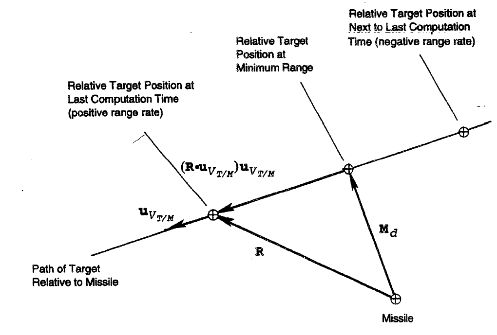
Figure 2: Miss-distance\(𝑀_𝑑\): miss distance vector at time of closet approach directed from missile to target
\(𝑅\): range vector
\(𝑢_{𝑉_{𝑇/𝑀}}\): unit vector in direction of relative velocity vector \(𝑉_{𝑇/𝑀}\)
6. Results#
Configure pyplot#
[31]:
from matplotlib import pyplot as plt
plt.style.use('dark_background')

fcsize = 4
fontsize = 5
linewidth = 1
asp = 1080 / 1920
plt.rcParams['figure.dpi'] = 300
plt.rcParams["font.family"] = 'Times New Roman'
plt.rcParams['figure.figsize'] = (fcsize, fcsize * asp)
plt.rcParams['figure.subplot.top'] = 0.9
plt.rcParams['figure.subplot.left'] = 0.15
plt.rcParams['figure.subplot.right'] = 0.9
plt.rcParams['figure.subplot.bottom'] = 0.2
plt.rcParams['figure.subplot.hspace'] = 0.8
Trajectories#
[32]:
plt.switch_backend('inline')
fig, (ax1, ax2) = plt.subplots(2, 1)

ax1.plot(missile.data('x', 1 / 1000)[1], missile.data('y', 1 / 1000)[1], 'b', linewidth = linewidth, label = 'missile')
ax1.plot(target.data('x', 1 / 1000)[1], target.data('y', 1 / 1000)[1], 'm', linewidth = linewidth, label = 'target')
c4d.plotdefaults(ax1, 'Top View', '', 'Crossrange (km)', fontsize = fontsize)

ax2.plot(missile.data('x', 1 / 1000)[1], -missile.data('z', 1 / 1000)[1], 'b', linewidth = linewidth, label = 'missile')
ax2.plot(target.data('x', 1 / 1000)[1], -target.data('z', 1 / 1000)[1], 'm', linewidth = linewidth, label = 'target')
c4d.plotdefaults(ax2, 'Side View', 'Downrange (km)', 'Altitude (km)', fontsize = fontsize)

plt.legend(fontsize = 4, facecolor = None, loc = 'lower right');
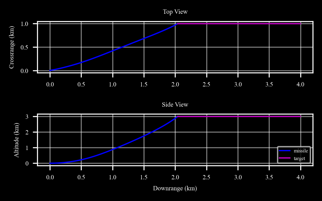
Figure 3: TrajectoriesEuler angles#
[33]:
_, ax = plt.subplots()

ax.plot(*missile.data('phi', c4d.r2d), 'b', linewidth = linewidth, label = '$\\varphi$')
ax.plot(*missile.data('theta', c4d.r2d), 'm', linewidth = linewidth, label = '$\\theta$')
ax.plot(*missile.data('psi', c4d.r2d), 'y', linewidth = linewidth, label = '$\\psi$')
c4d.plotdefaults(ax, 'Euler Angles', 'Time[s]', '[deg]', fontsize = fontsize)

plt.legend(fontsize = 4, facecolor = None, loc = 'lower right');
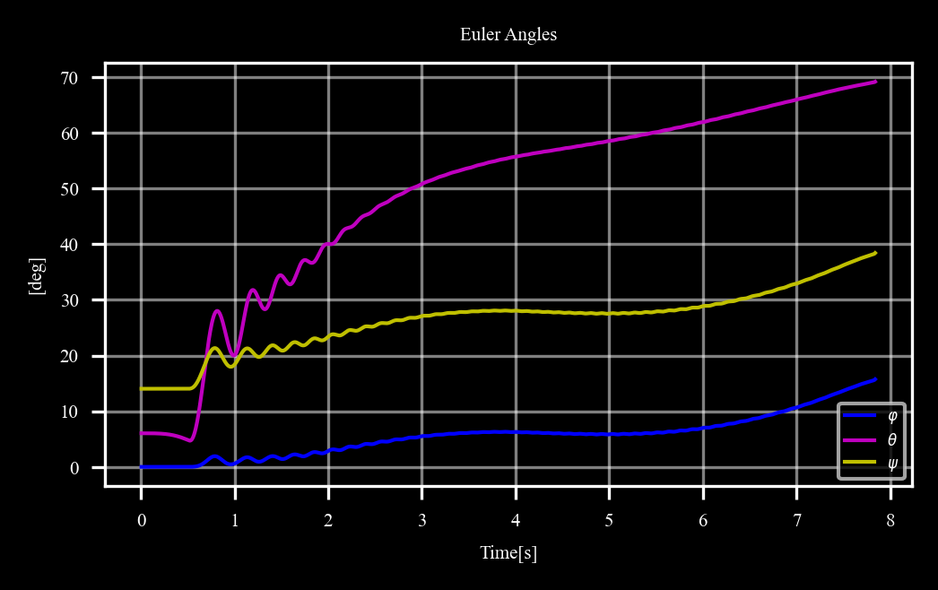
Figure 4: Euler AnglesLine-of-sight rates#
[34]:
# omega los
fig, (ax1, ax2) = plt.subplots(2, 1)
ax1.plot(missile.data('t'), np.array(omegaf_data)[:, 0] * c4d.r2d, 'm', linewidth = linewidth)
ax2.plot(missile.data('t'), np.array(omegaf_data)[:, 1] * c4d.r2d, 'm', linewidth = linewidth)
ax1.set_ylim(0, 3.5)
ax2.set_ylim(-0.25, 0.6)
c4d.plotdefaults(ax1, '$\\omega_{pitch}$', fontsize = fontsize)
c4d.plotdefaults(ax2, '$\\omega_{yaw}$', 'Time (s)', fontsize = fontsize)
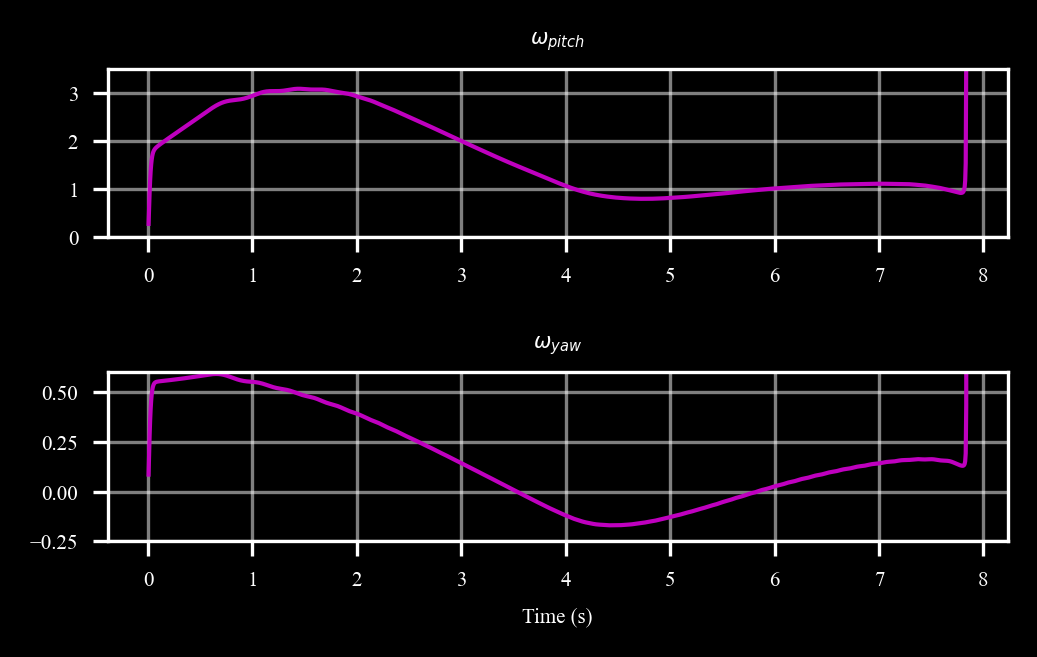
Figure 5: Line-Of-Sight Rates7. Provision for Monte Carlo Simulation#
While this simulation demonstrates the development and testing of a guidance system, future work can explore the system’s sensitivity to internal modeling errors.
In this implementation, the main loop was executed using a fixed sample of the seeker’s random variables, the time constants (\(\tau_1\), \(\tau_2\)), which influence the accuracy of the LOS rate measurements.
A Monte Carlo simulation can be conducted to evaluate how variability in these time constants affects system performance.
By introducing random variations within reasonable bounds for \(\tau_1\) and \(\tau_2\), one can assess the robustness of the guidance algorithm and its tolerance to modeling inaccuracies and hardware imperfections.
8. Summary#
This 6DOF missile guidance simulation models the flight dynamics of a missile pursuing a non-maneuvering target, achieving a precise miss distance through the proportional navigation guidance algorithms. The simulation integrates translational and rotational equations of motion, accounts for aerodynamic forces, propulsion, and gravity, and employs a line-of-sight seeker to generate control commands.
Trajectory plots and Euler angle visualizations reveal the missile’s dynamic behavior, offering insights into guidance system performance.
Future enhancements could incorporate maneuvering targets or environmental effects to broaden the simulation’s applicability.
References#
1 Missile Flight Simulation Part One Surface-to-Air Missiles, MIL-HDBK-1211(MI) 17 July 1995. In: Military Handbook, 1995.