Kalman#
- class c4dynamics.filters.kalman.kalman(X: dict, F: ndarray, H: ndarray, steadystate: bool = False, G: ndarray | None = None, P0: ndarray | None = None, Q: ndarray | None = None, R: ndarray | None = None)[source]#
Kalman Filter.
Discrete linear Kalman filter class for state estimation.
kalmanprovides methods for prediction and update (correct) phases of the filter.For background material, implementation, and examples, please refer to
filters.- Parameters:
X (dict) – Initial state variables and their values.
F (numpy.ndarray) – Discrete-time state transition matrix. Defaults to None.
H (numpy.ndarray) – Discrete-time measurement matrix. Defaults to None.
steadystate (bool, optional) – Flag to indicate if the filter is in steady-state mode. Defaults to False.
G (numpy.ndarray, optional) – Discrete-time control matrix. Defaults to None.
P0 (numpy.ndarray, optional) – Covariance matrix, or standard deviations array, of the initial estimation error. Mandatory if steadystate is False. If P0 is one-dimensional array, standard deviation values are expected. Otherwise, variance values are expected.
Q (numpy.ndarray, optional) – Process noise covariance matrix. Defaults to None.
R (numpy.ndarray, optional) – Measurement noise covariance matrix. Defaults to None.
Notes
1. kalman is a subclass of
state, as such the variables provided within the parameter X form its state variables. Hence, X is a dictionary of variables and their initial values, for example:X = {'x': x0, 'y': y0, 'z': z0}.2. Steady-state mode: if the underlying system is linear time-invariant (LTI), and the noise covariance matrices are time-invariant, then a steady-state mode of the Kalman filter can be employed. In steady-state mode the Kalman gain (K) and the estimation covariance matrix (P) are computed once and remain constant (‘steady-state’) for the entire run-time, performing as well as the time-varying filter. Note however that also in steady-state mode the predict and the update steps are separated and the user must call each of them at a time.
- Raises:
TypeError: – If X is not a dictionary.
ValueError: – If P0 is not provided when steadystate is False.
ValueError: – If system matrices are not fully provided.
Examples
The examples in the introduction to the
filtersmodule demonstrate the operations of the Kalman filter for inputs from electromagnetic devices, such as an altimeter, which measures the altitude.An accurate Japaneese train travels 150 meters in one second (\(F = 1, u = 1, G = 150, Q = 0.05\)). A sensor measures the train position with noise variance of \(200m^2\) (\(H = 1, R = 200\)). The initial position of the train is known with uncertainty of \(0.5m\) (\(P0 = 0.5^2\)).
Note
The system may be interpreted as follows:
\(F = 1\) - constant position
\(u = 1, G = 150\) - constant velocity control input
The advantage of this model is in its being first order. However, a slight difference between the actual dynamics and the modeled process will result in a lag with the tracked object.
Import required packages:
>>> from c4dynamics.filters import kalman
>>> from matplotlib import pyplot as plt
>>> import c4dynamics as c4d
Let’s run a filter.
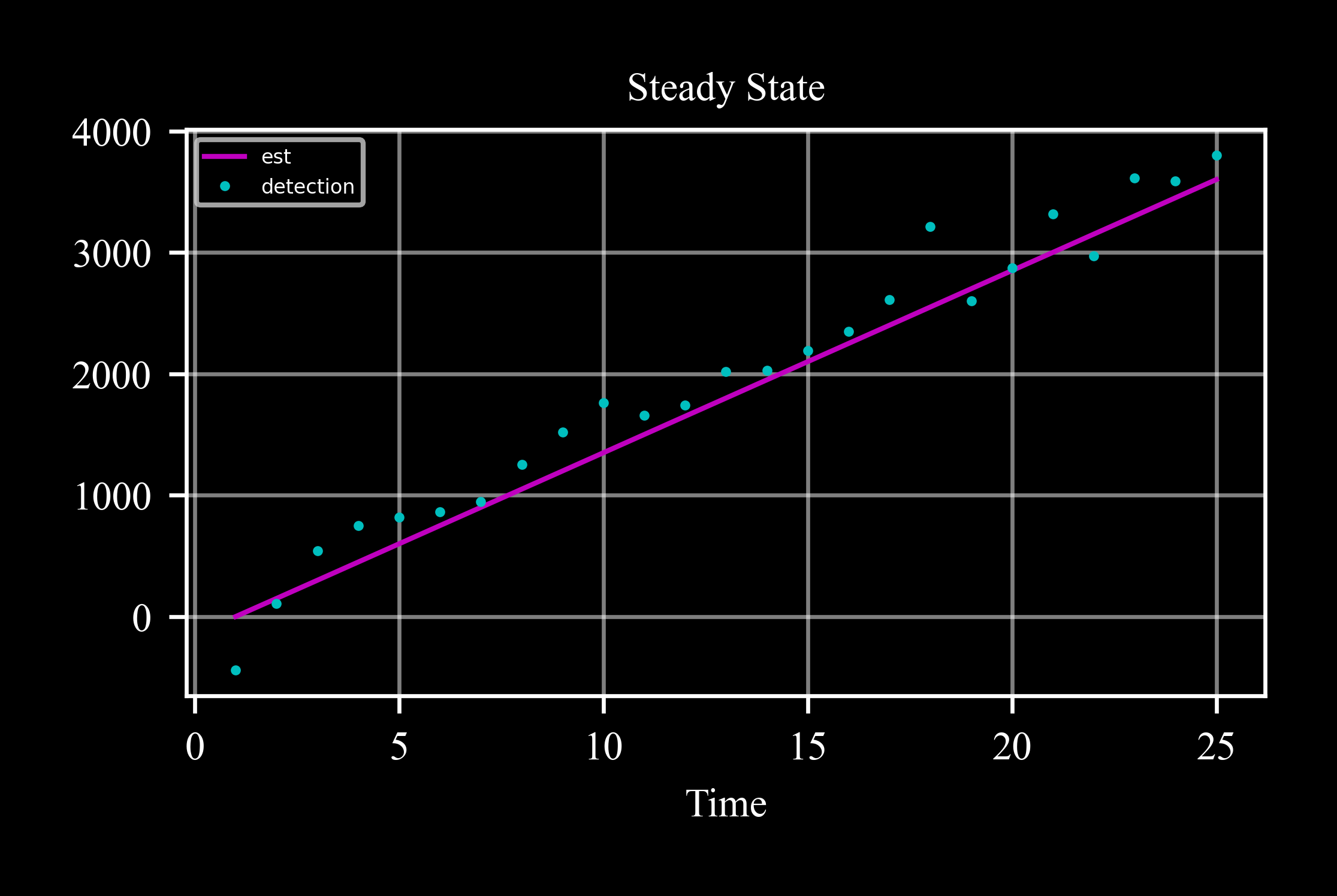
First, since the covariance matrices are constant we can utilize the steady state mode of the filter. This requires initalization with the respective flag:
>>> v = 150
>>> sensor_noise = 200
>>> kf = kalman({'x': 0}, P0 = 0.5**2, F = 1, G = v, H = 1
...                         , Q = 0.05, R = sensor_noise**2, steadystate = True)
>>> for t in range(1, 26): #  seconds.
...   # store for later
...   kf.store(t)
...   # predict + correct
...   kf.predict(u = 1)
...   kf.detect = v * t + np.random.randn() * sensor_noise
...   kf.storeparams('detect', t)
Recall that a
kalmanobject, as subclass of thestate, encapsulates the process state vector:>>> print(kf) [ x ]
It can also employ the
plotor any other method of the state class:>>> kf.plot('x') >>> plt.gca().plot(*kf.data('detect'), 'co', label = 'detection') >>> plt.gca().legend() >>> plt.show()
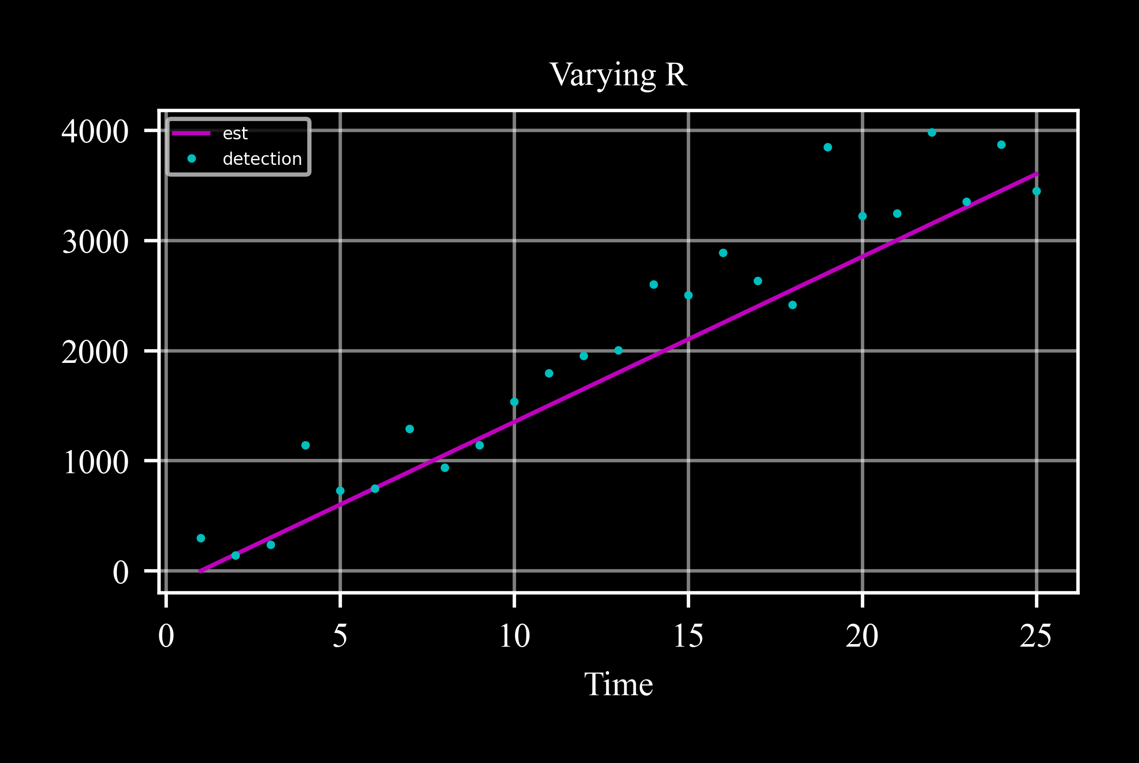
Let’s now assume that as the train moves farther from the station, the sensor measurements degrade.
The measurement covariance matrix therefore increases accordingly, and the steady state mode cannot be used:
>>> v = 150
>>> kf = kalman({'x': 0}, P0 = 0.5*2, F = 1, G = v, H = 1, Q = 0.05)
>>> for t in range(1, 26): #  seconds.
...   kf.store(t)
...   sensor_noise = 200 + 8 * t
...   kf.predict(u = 1)
...   kf.detect = v * t + np.random.randn() * sensor_noise
...   kf.K = kf.update(kf.detect, R = sensor_noise**2)
...   kf.storeparams('detect', t)
Methods
kalman.predict([u, Q])Predicts the filter's next state and covariance matrix based on the current state and the process model.
kalman.update(z[, R])Updates (corrects) the state estimate based on the given measurements.
kalman.store([t])Stores the current state and diagonal elements of the covariance matrix.