c4dynamics.sensors.seeker.seeker.bias

property seeker.bias: float

Gets and sets the object’s bias.

The bias is a random variable generated once at the stage of constructing the instance by the errors model:

\[bias = std \cdot randn\]

Where bias_std is a parameter with default value of 0.1° for seeker object, and 0.3° for radar object.

To get the bias generated by the errors model, or to override it, the user may call bias to get or set the final bias error.

Parameters:

bias (float) – Required bias, [radians].

Returns:

bias (float) – Current bias, [radians].

Example

The following example for a seeker object is directly applicable to a radar object too. Simply replace c4d.sensors.seeker(origin = pedestal,...) with c4d.sensors.radar(origin = pedestal,...).

Required packages:

>>> import c4dynamics as c4d
>>> from matplotlib import pyplot as plt
>>> import numpy as np

Settings and initial conditions:

(see seeker examples for more details):

Target:

>>> tgt = c4d.datapoint(x = 1000, y = 0, vx = -80 * c4d.kmh2ms, vy = 10 * c4d.kmh2ms)
>>> for t in np.arange(0, 60, 0.01):
...   tgt.inteqm(np.zeros(3), .01) 
...   tgt.store(t)

Origin:

>>> pedestal = c4d.rigidbody(z = 30, theta = -1 * c4d.d2r)

Ground truth reference:

>>> skr_ideal = c4d.sensors.seeker(origin = pedestal, isideal = True)

Tracking with bias

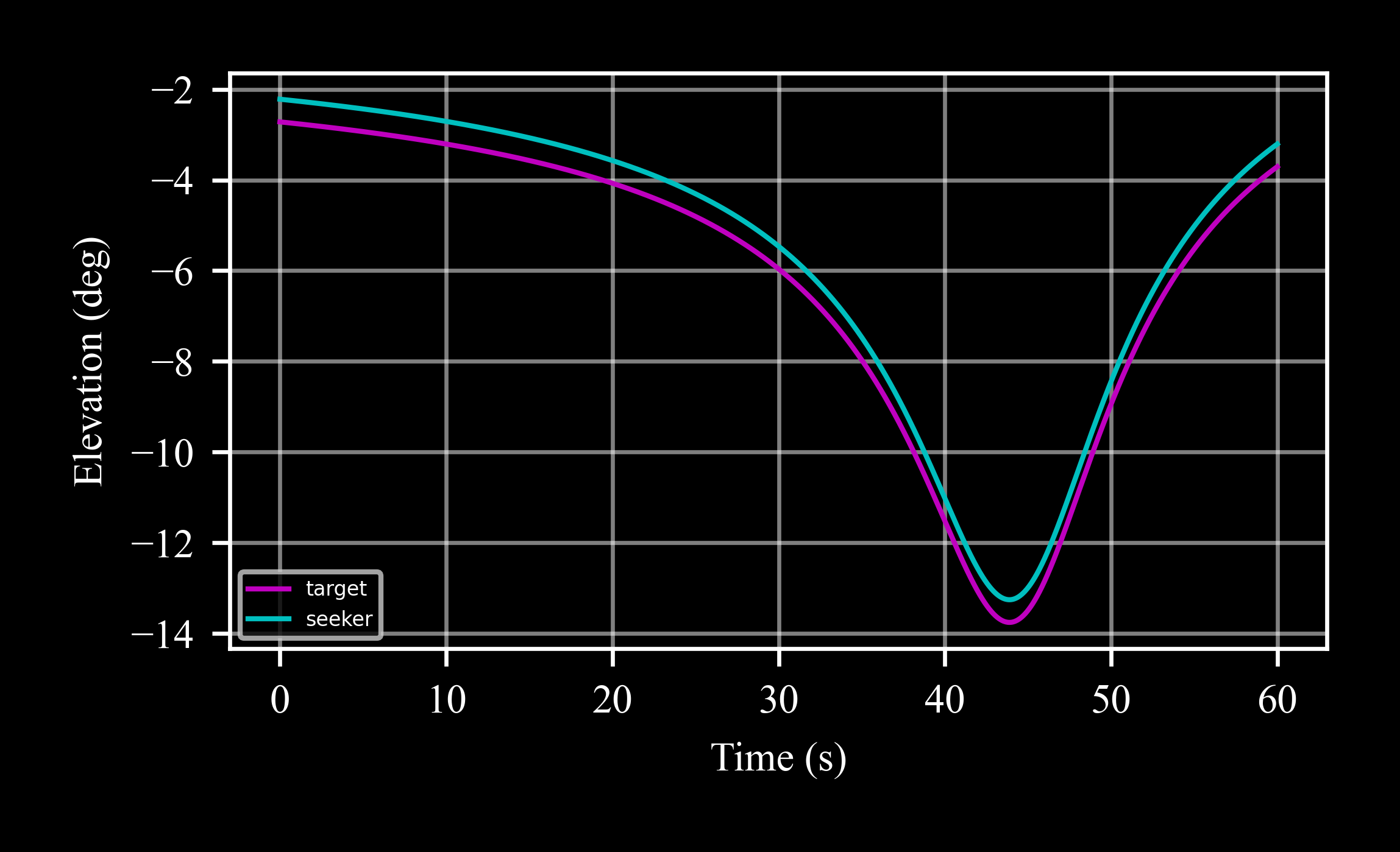
Define a seeker with a bias error only (mute the scale factor and the noise) and set it to 0.5° to track a constant velocity target:

>>> skr = c4d.sensors.seeker(origin = pedestal, scale_factor_std = 0, noise_std = 0)
>>> skr.bias = .5 * c4d.d2r
>>> for x in tgt.data():
...   skr_ideal.measure(c4d.create(x[1:]), t = x[0], store = True)  
...   skr.measure(c4d.create(x[1:]), t = x[0], store = True)  

Compare the biased seeker with the true target angles (ideal seeker):

>>> ax = plt.subplot()
>>> ax.plot(*skr_ideal.data('el', scale = c4d.r2d), label = 'target')  
>>> ax.plot(*skr.data('el', scale = c4d.r2d), label = 'seeker')  

Example

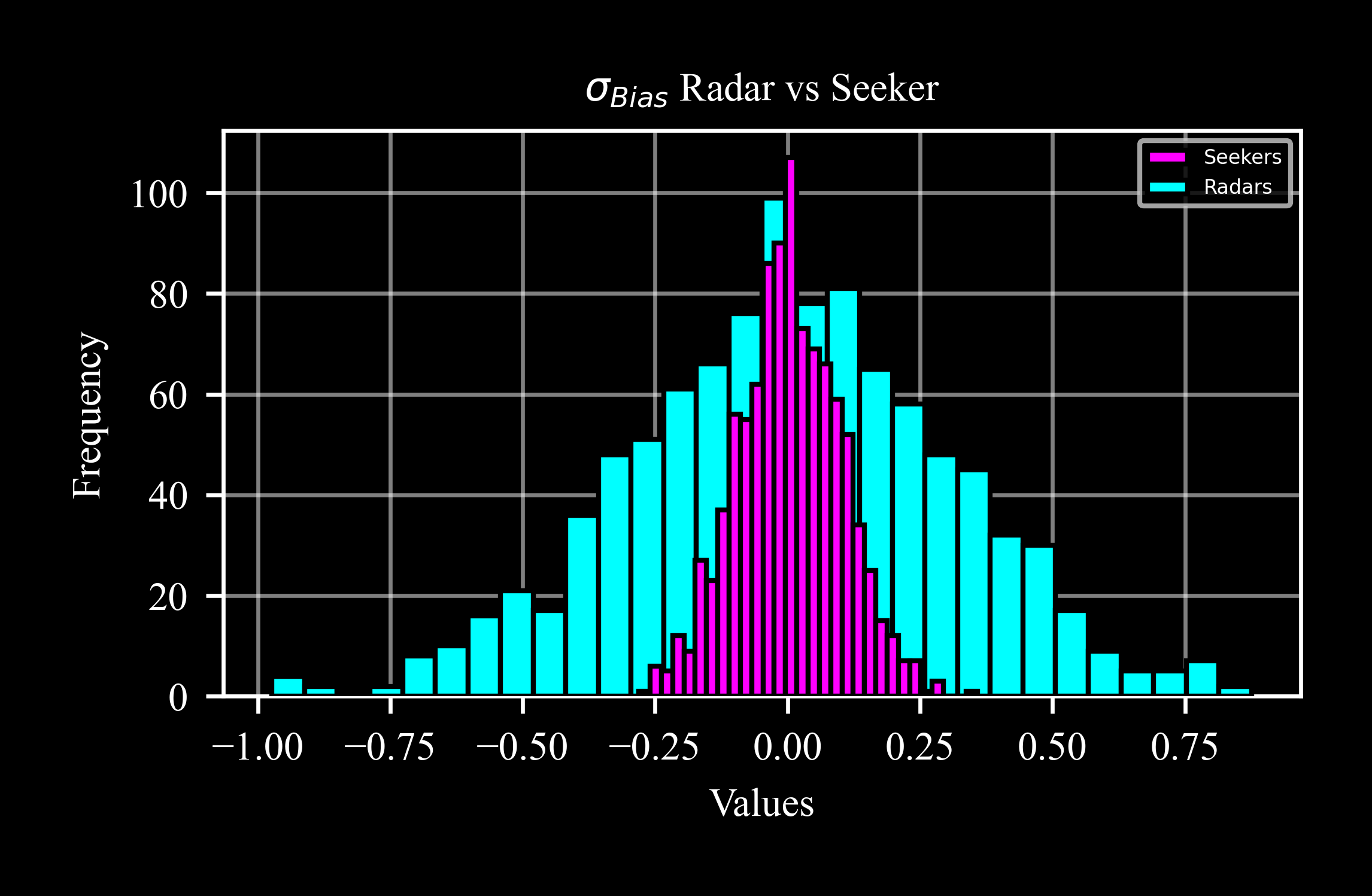
The distribution of normally generated random variables is characterized by its bell-shaped curve, which is symmetric about the mean. The area under the curve represents probability, with about 68% of the data falling within one standard deviation (1σ) of the mean, 95% within two, and 99.7% within three, making it a useful tool for understanding and predicting data behavior.

In radar objects, and seeker objects in general, the bias and scale factor vary among different instances to allow a realistic simulation of performance behavior in a technique known as Monte Carlo.

Let’s examine the bias distribution across mutliple radar instances with a default bias_std = 0.3° in comparison to seeker instances with a default bias_std = 0.1°:

>>> from c4dynamics.sensors import seeker, radar
>>> seekers = []
>>> radars = []
>>> for i in range(1000):
...   seekers.append(seeker().bias * c4d.r2d)
...   radars.append(radar().bias * c4d.r2d)

The histogram highlights the broadening of the distribution as the standard deviation increases:

>>> ax = plt.subplot()
>>> ax.hist(seekers, 30, label = 'Seekers') 
>>> ax.hist(radars, 30, label = 'Radars')