c4dynamics.rotmat.animate.animate

c4dynamics.rotmat.animate.animate#

Animate a rigidbody.

Animates the rigid body’s motion using a 3D model according to the 3-2-1 Euler angles histories.

Important Note

Using the animate function requires installation of Open3D which is not a prerequisite of C4dynamics. For the different ways to install Open3D please refer to its official website. A direct installation with pip:

pip install open3d

Parameters:

modelpath (str) – A path to a single file model or a path to a folder containing multiple model files. If the provided path is of a folder, only model files should exist in it. Typically supported files for mesh models are .obj, .stl, .ply. Supported point cloud file is .pcd. If your point cloud file has .ply extension, convert it to a .pcd first. You may do that by using Open3D, see note below.
angle0 (array_like, optional) – Initial Euler angles \([\varphi, \theta, \psi]\), in radians, representing the model attitude with respect to the screen frame, see note below.
modelcolor (array_like, optional) – Colors array [R, G, B] of values between 0 and 1. The shape of modelcolor is mx3, where m is either 1 or as the number of the model files. If m > 1, then the order of the colors in the array should match the alphabetical order of the files in modelpath.
dt (float, optional) – Time step between two frames for the animation. Default is 1msec.
savedir (str, optional) – If provided, saves each frame as an image in the specified directory. Default is None.

Note

Currently, only 321 Euler order of rotation is supported. Therefore if the stored angular state is produced by using other set of Euler angles, they have to be converted to a 321 set first.
If the provided path is of a folder, only model files should exist in it. Typically supported files for mesh models are .obj, .stl, .ply. Supported point cloud file is .pcd. If your point cloud file has .ply extension, convert it to a .pcd first. You may do that by using Open3D:
```
>>> import open3d as o3d
>>> pcd = o3d.io.read_point_cloud('model.ply') 
>>> o3d.io.write_point_cloud('model.pcd', pcd) 
```
For more info see Open3D documentation
Initial Euler angles \([\varphi, \theta, \psi]\), in radians, representing the model attitude with respect to the screen frame, see note below. The screen frame is defined as follows:
```
x: right
y: up
z: outside
```
Default attitude [0, 0, 0].

Examples

The 3D models used in the following examples can be downloaded and fetched by c4dynamics’ datasets:

>>> import c4dynamics as c4d

>>> bunnypath = c4d.datasets.d3_model('bunny') # 'bunny.pcd': point cloud data file
Fetched successfully
>>> bunnymesh_path = c4d.datasets.d3_model('bunnymesh') # 'bunny_mesh.ply': polygon file
Fetched successfully
>>> f16path = c4d.datasets.d3_model('f16') # folder of 10 stl files.
Fetched successfully

For more details, refer to c4dynamics.datasets.

Animate Stanford bunny

1. The Stanford bunny is a computer graphics 3D test model developed by Greg Turk and Marc Levoy in 1994 at Stanford University. The model consists of 69,451 triangles, with the data determined by 3D scanning a ceramic figurine of a rabbit. For more details, refer to The Stanford 3D Scanning Repository

>>> bunny = c4d.rigidbody()
>>> # generate an arbitrary attitude motion
>>> dt = 0.01
>>> T = 5
>>> for t in np.arange(0, T, dt):
...   bunny.psi += dt * 360 * c4d.d2r / T
...   bunny.store(t)
>>> bunny.animate(bunnypath, cbackground = [0, 0, 0])

2. You can change the model’s color by setting the modelcolor parameter. Here is an example of a mesh version of Stanford bunny with a custom color:

>>> bunny.animate(bunnymesh_path, cbackground = [0, 0, 0], modelcolor = [1, 0, .5])

Motion of a dynamic system

An F16 has the following Euler angles:

>>> f16 = c4d.rigidbody()
>>> dt = 0.01
>>> for t in np.arange(0, 9, dt):
...   if t < 3:
...     f16.psi += dt * 180 * c4d.d2r / 3
...   elif t < 6:
...     f16.theta += dt * 180 * c4d.d2r / 3
...   else:
...     f16.phi -= dt * 180 * c4d.d2r / 3
...   f16.store(t)

The jet model is consisted of multiple files, therefore the f16 rigidbody object that was simulated with the above motion is provided with a path to the consisting folder.

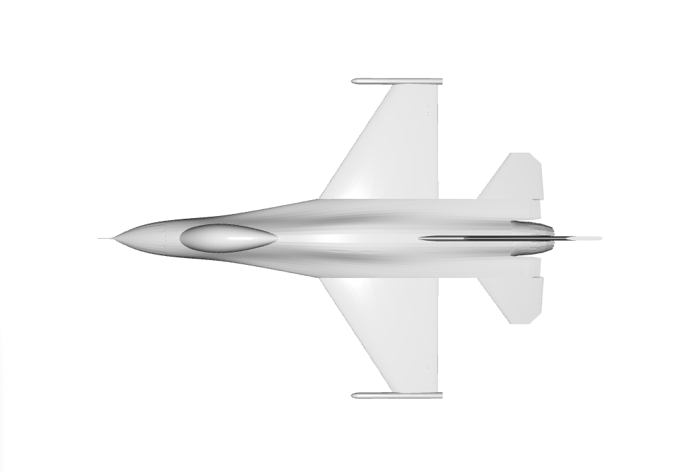
>>> f16.animate(f16path)

4. It’s obvious that the animated model doesn’t follow the required rotation as simulated above. This because the model initial postion isn’t aligned with the screen frame. To align the aircraft body frame which defined as:

x: centerline
z: perpendicular to x, downward
y: completes the right-hand coordinate system

With the screen frame which defined as:

x: rightward
y: upward
z: outside the screen

We should examine a frame of the model before any rotation. It can be achieved by using Open3D:

>>> import os
>>> import open3d as o3d

>>> model = []
>>> for f in sorted(os.listdir(f16path)):
...   mfilepath = os.path.join(f16path, f)
...   m = o3d.io.read_triangle_mesh(mfilepath)
...   m.compute_vertex_normals() 
...   model.append(m)
>>> o3d.visualization.draw_geometries(model)

It turns out that for 3-2-1 order of rotation (see rotmat) the body frame with respect to the screen frame is given by:

Rotation of 180deg about y (up the screen)
Rotation of 90deg about x (right the screen)

Let’s re-run with the correct initial conditions:

>>> x0 = [90 * c4d.d2r, 0, 180 * c4d.d2r]
>>> f16.animate(f16path, angle0 = x0)

5. The attitude is correct but the the model is colorless. Let’s give it some color; We sort the colors by the jet’s parts alphabetically as it assigns the values according to the order of an alphabetical reading of the files in the folder. Finally convert it to a list.

>>> f16colors = list({'Aileron_A_F16':     [0.3 * 0.8, 0.3 * 0.8, 0.3 * 1]
...                 , 'Aileron_B_F16':     [0.3 * 0.8, 0.3 * 0.8, 0.3 * 1]
...                 , 'Body_F16':          [0.8, 0.8, 0.8]
...                 , 'Cockpit_F16':       [0.1, 0.1, 0.1]
...                 , 'LE_Slat_A_F16':     [0.3 * 0.8, 0.3 * 0.8, 0.3 * 1]
...                 , 'LE_Slat_B_F16':     [0.3 * 0.8, 0.3 * 0.8, 0.3 * 1]
...                     , 'Rudder_F16':        [0.3 * 0.8, 0.3 * 0.8, 0.3 * 1]
...                       , 'Stabilator_A_F16':  [0.3 * 0.8, 0.3 * 0.8, 0.3 * 1]
...                          , 'Stabilator_B_F16':  [0.3 * 0.8, 0.3 * 0.8, 0.3 * 1]
...                 }.values())
>>> f16.animate(f16path, angle0 = x0, modelcolor = f16colors)

It can also be painted with a single color for all its parts and a single color for the background:

>>> f16.animate(f16path, angle0 = x0, modelcolor = [0, 0, 0], cbackground = np.array([230, 230, 255]) / 255)

Finally, let’s use the savedir option using the c4dynamics’ gif util to generate a gif file out of the model animation

>>> f16colors = np.vstack(([255, 215, 0], [255, 215, 0]
...                         , [184, 134, 11], [0, 32, 38]
...                             , [218, 165, 32], [218, 165, 32], [54, 69, 79]
...                                 , [205, 149, 12], [205, 149, 12])) / 255
>>> outfol = os.path.join('tests', '_out', 'f16a')
>>> f16.animate(f16path, angle0 = x0, savedir = outfol, modelcolor = f16colors)
>>> # the storage folder 'outfol' is the source of images for the gif function
>>> # the 'duration' parameter sets the required length of the animation
>>> gifname = 'f16_animation.gif'
>>> c4d.gif(outfol, gifname, duration = 1)

Viewing the gif on a Jupyter notebook is possible by using the Image funtion of the IPython module:

>>> import os
>>> from IPython.display import Image

>>> gifpath = os.path.join(outfol, gifname)
>>> Image(filename = gifpath) 

c4dynamics.rotmat.animate.animate

Contents

c4dynamics.rotmat.animate.animate#