c4dynamics.eqm.derivs.eqm3

c4dynamics.eqm.derivs.eqm3(dp: datapoint, F: ndarray | list) → ndarray

Translational motion derivatives.

These equations represent a set of first-order ordinary differential equations (ODEs) that describe the motion of a datapoint in three-dimensional space under the influence of external forces.

Parameters:

• dp (datapoint) – C4dynamics’ datapoint object for which the equations of motion are calculated.

• F (array_like) – Force vector \([F_x, F_y, F_z]\)

Returns:

out (numpy.array) – \([dx, dy, dz, dv_x, dv_y, dv_z]\) 6 derivatives of the equations of motion, 3 position derivatives, and 3 velocity derivatives.

Examples

Import required packages:

>>> import c4dynamics as c4d
>>> from matplotlib import pyplot as plt
>>> import numpy as np

>>> dp = c4d.datapoint()
>>> dp.mass = 10                    # mass 10kg     
>>> F  = [0, 0, c4d.g_ms2]          # g_ms2 = 9.8m/s^2
>>> c4d.eqm.eqm3(dp, F)             
array([0  0  0  0  0  0.980665])

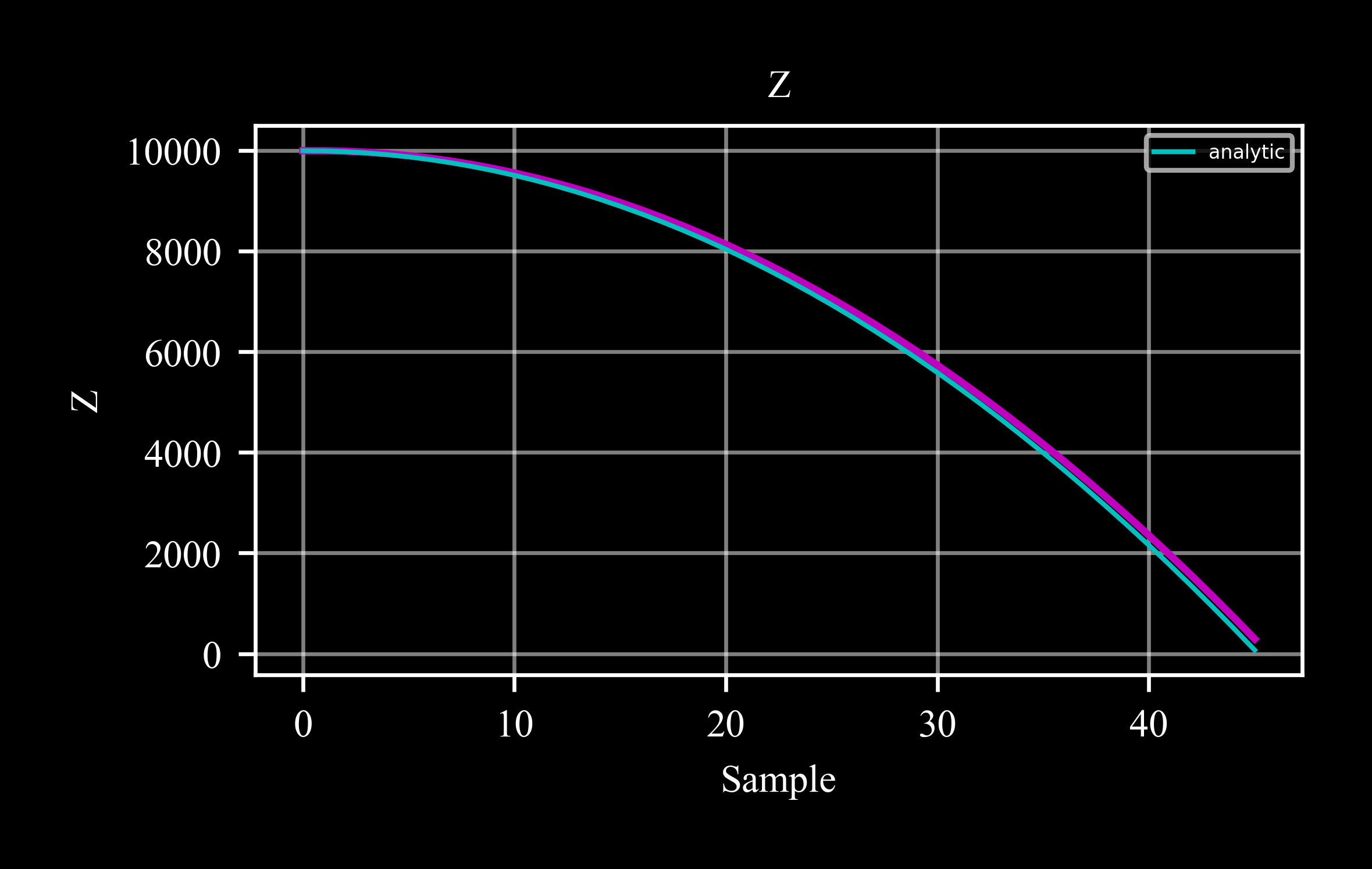
Euler integration on the equations of motion of mass in a free fall:

>>> h0 = 10000
>>> pt = c4d.datapoint(z = 10000)
>>> while pt.z > 0:
...   pt.store()
...   dx = c4d.eqm.eqm3(pt, [0, 0, -c4d.g_ms2])
...   pt.X += dx  # (dt = 1)
>>> pt.plot('z')
>>> # comapre to anayltic solution
>>> t = np.arange(len(pt.data('t')))
>>> z = h0 - .5 * c4d.g_ms2 * t**2
>>> plt.gca().plot(t[z > 0], z[z > 0], 'c', linewidth = 1)