c4dynamics.eqm.integrate.int6#
- c4dynamics.eqm.integrate.int6(rb: rigidbody, forces: ndarray | list, moments: ndarray | list, dt: float, derivs_out: bool = False) ndarray[tuple[Any, ...], dtype[float64]] | Tuple[ndarray[tuple[Any, ...], dtype[float64]], ndarray[tuple[Any, ...], dtype[float64]]][source]#
A step integration of the equations of motion.
This method makes a numerical integration using the fourth-order Runge-Kutta method.
The integrated derivatives are of three dimensional translational motion as given by
eqm6.The result is an integrated state in a single interval of time where the size of the step is determined by the parameter dt.
- Parameters:
dp (
datapoint) – The datapoint which state vector is to be integrated.forces (numpy.array or list) – An external forces array acting on the body.
dt (float) – Time step for integration.
derivs_out (bool, optional) – If true, returns the last three derivatives as an estimation for the acceleration of the datapoint.
- Returns:
X (numpy.float64) – An integrated state.
dxdt4 (numpy.float64, optional) – The last six derivatives of the equations of motion. These derivatives can use as an estimation for the translational and angular acceleration of the datapoint. Returned if derivs_out is set to True.
Algorithm
The integration steps follow the Runge-Kutta method:
Compute k1 = f(ti, yi)
Compute k2 = f(ti + dt / 2, yi + dt * k1 / 2)
Compute k3 = f(ti + dt / 2, yi + dt * k2 / 2)
Compute k4 = f(ti + dt, yi + dt * k3)
Update yi = yi + dt / 6 * (k1 + 2 * k2 + 2 * k3 + k4)
Examples
In the following example, the equations of motion of a cylinderical body are integrated by using the
int6.The results are compared to the results of the same equations integrated by using scipy.odeint.
int6
Import required packages
>>> import c4dynamics as c4d
>>> from matplotlib import pyplot as plt
>>> from scipy.integrate import odeint
>>> import numpy as np
Settings and initial conditions
>>> dt = 0.5e-3
>>> t  = np.arange(0, 10, dt)
>>> theta0 =  80 * c4d.d2r       # deg
>>> q0     =  0 * c4d.d2r        # deg to sec
>>> Iyy    =  .4                 # kg * m^2
>>> length =  1                  # meter
>>> mass   =  0.5                # kg
Define the cylinderical-rigidbody object
>>> rb = c4d.rigidbody(theta = theta0, q = q0)
>>> rb.I = [0, Iyy, 0]
>>> rb.mass = mass
Main loop:
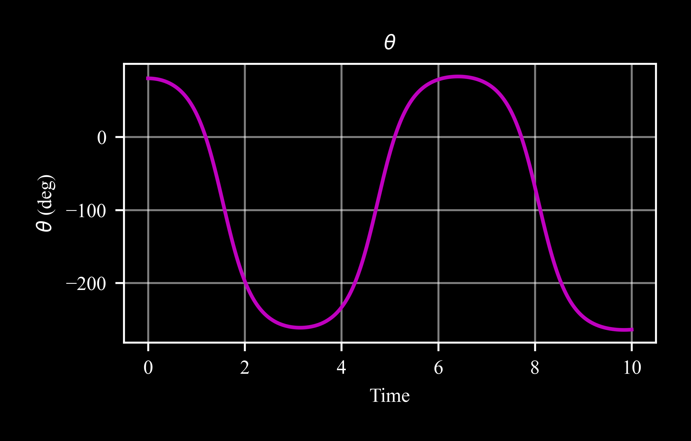
>>> for ti in t:
...   rb.store(ti)
...   tau_g = -rb.mass * c4d.g_ms2 * length / 2 * c4d.cos(rb.theta)
...   rb.X = c4d.eqm.int6(rb, np.zeros(3), [0, tau_g, 0], dt)
>>> rb.plot('theta')
scipy.odeint
>>> def pend(y, t):
...  theta, omega = y
...  dydt = [omega, -rb.mass * c4d.g_ms2 * length / 2 * c4d.cos(theta) / Iyy]
...  return dydt
>>> sol = odeint(pend, [theta0, q0], t)
Compare to int6:
>>> plt.plot(*rb.data('theta', c4d.r2d), 'm', label = 'c4dynamics.int6')
>>> plt.plot(t, sol[:, 0] * c4d.r2d, 'c', label = 'scipy.odeint')
>>> c4d.plotdefaults(plt.gca(), 'Equations of Motion Integration ($\theta$)', 'Time', 'degrees', fontsize = 12)
>>> plt.legend()
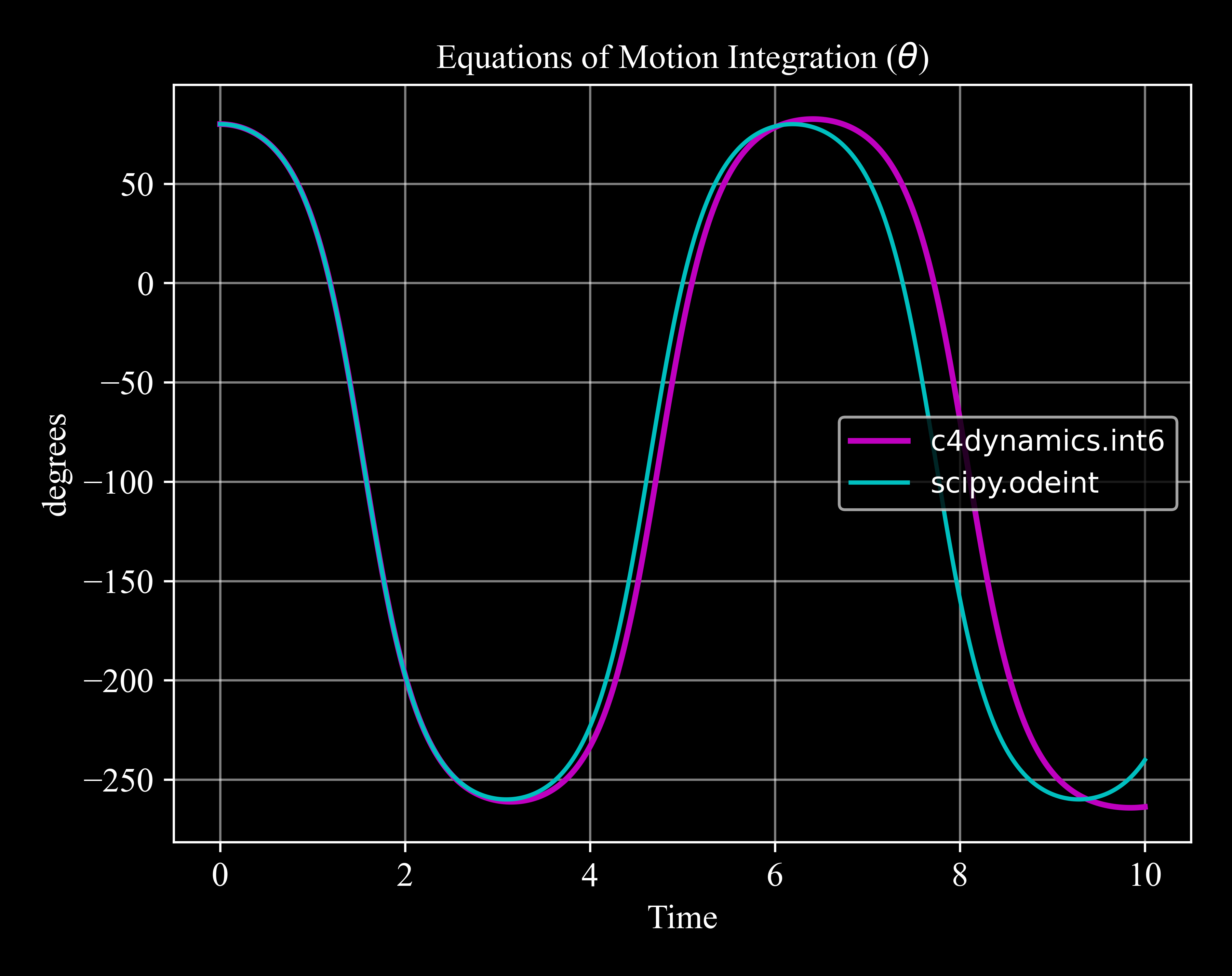
Note - Differences Between Scipy and C4dynamics Integration
The difference in the results derive from the method of delivering the forces and moments. scipy.odeint gets as input the function that caluclates the derivatives, where the forces and moments are included in it:
dydt = [omega, -rb.mass * c4d.g_ms2 * length / 2 * c4d.cos(theta) / Iyy]
This way, the forces and moments are recalculated for each step of the integration.
c4dynamics.eqm.int6 on the other hand, gets the vectors of forces and moments only once when the function is called and therefore refer to them as constant for the four steps of integration.
When external factors may vary quickly over time and a high level of accuracy is required, using other methods, like scipy.odeint, is recommanded. If computational resources are available, a decrement of the step-size may be a workaround to achieve high accuracy results.