c4dynamics.sensors.radar.radar.measure

radar.measure(target: state, t: float = -1, store: bool = False) → tuple[float | None, float | None, float | None]

Measures range, azimuth and elevation between the radar and a target.

If the radar time-constant dt was provided when the radar was created, then measure returns None for any t < last_t + dt, where t is the time input, last_t is the last measurement time, and dt is the radar time-constant. Default behavior, returns measurements for each call.

If store = True, the method stores the measured azimuth and elevation along with a timestamp (t = -1 by default, if not provided otherwise).

Parameters:

• target (state) – A Cartesian state object to measure by the radar, including at least one position coordinate (x, y, z).

• store (bool, optional) – A flag indicating whether to store the measured values. Defaults False.

• t (float, optional) – Timestamp [seconds]. Defaults -1.

Returns:

out (tuple) – range [meters, float], azimuth and elevation, [radians, float].

Raises:

ValueError – If target doesn’t include any position coordinate (x, y, z).

Example

measure in a program simulating real-time tracking of a constant velcoity target.

The target is represented by a datapoint and is simulated using the eqm module, which integrating the point-mass equations of motion.

An ideal radar uses as reference to the true position of the target.

At each cycle, the the radars take measurements and store the samples for later use in plotting the results.

Import required packages:

>>> import c4dynamics as c4d
>>> from matplotlib import pyplot as plt
>>> import numpy as np

Settings and initial conditions:

>>> dt = 0.01
>>> np.random.seed(321)
>>> tgt = c4d.datapoint(x = 1000, vx = -80 * c4d.kmh2ms, vy = 10 * c4d.kmh2ms)
>>> pedestal = c4d.rigidbody(z = 30, theta = -1 * c4d.d2r)
>>> rdr = c4d.sensors.radar(origin = pedestal, dt = 0.05)
>>> rdr_ideal = c4d.sensors.radar(origin = pedestal, isideal = True)

Main loop:

>>> for t in np.arange(0, 60, dt):
...   tgt.inteqm(np.zeros(3), dt)  
...   rdr_ideal.measure(tgt, t = t, store = True)    
...   rdr.measure(tgt, t = t, store = True)    
...   tgt.store(t)

Before viewing the results, let’s examine the error parameters generated by the errors model (c4d.r2d converts radians to degrees):

>>> rdr.rng_noise_std
1.0
>>> rdr.bias * c4d.r2d 
0.49...
>>> rdr.scale_factor 
1.01...
>>> rdr.noise_std * c4d.r2d
0.8

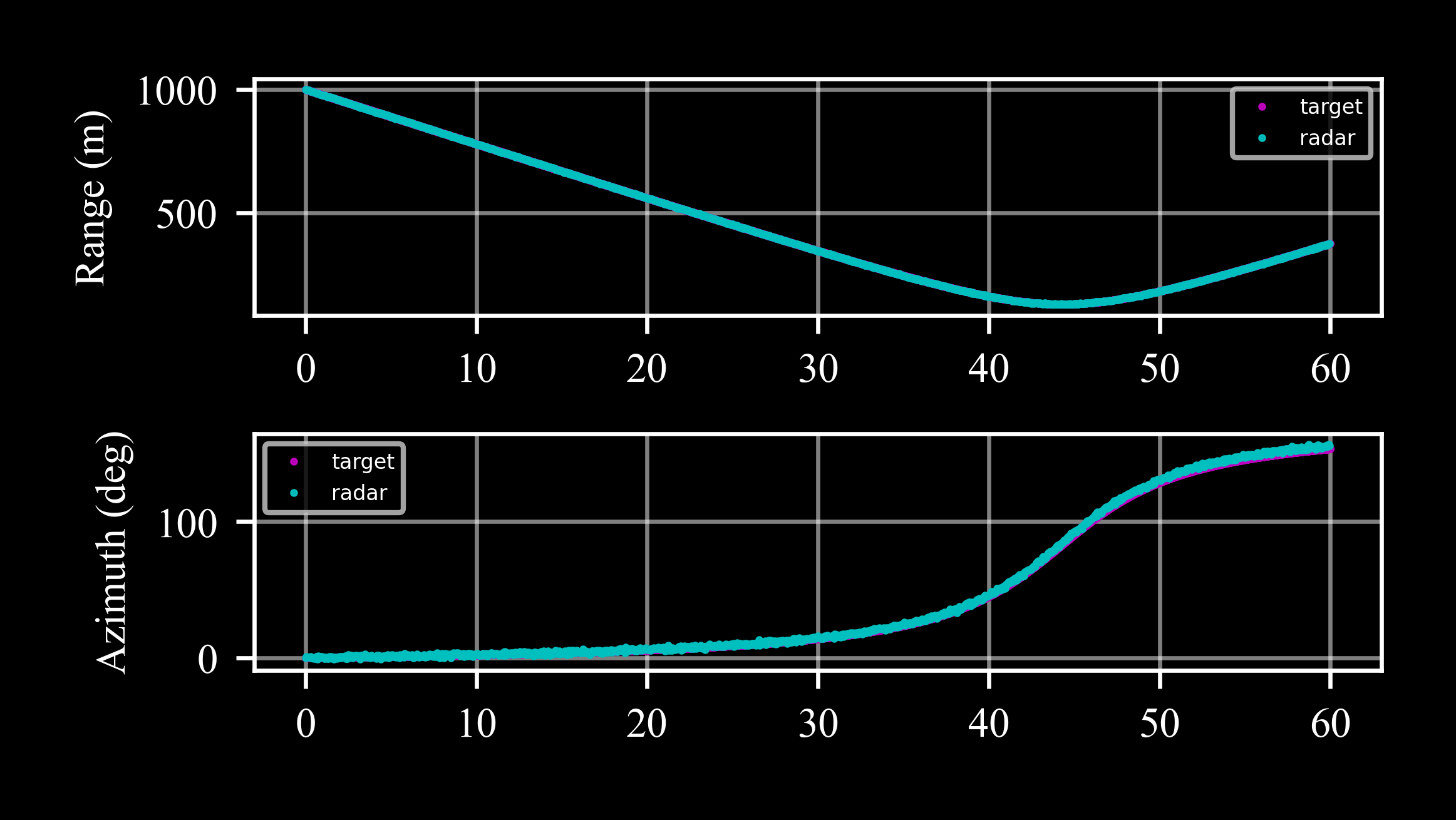
Then we excpect a constant bias of -0.02° and a ‘compression’ or ‘squeeze’ of 5% with respect to the target (as represented by the ideal radar):

>>> _, axs = plt.subplots(2, 1)  
>>> # range
>>> axs[0].plot(*rdr_ideal.data('range'), '.m', label = 'target')  
>>> axs[0].plot(*rdr.data('range'), '.c', label = 'radar')  
>>> # angles
>>> axs[1].plot(*rdr_ideal.data('az', scale = c4d.r2d), '.m', label = 'target')  
>>> axs[1].plot(*rdr.data('az', scale = c4d.r2d), '.c', label = 'radar')  

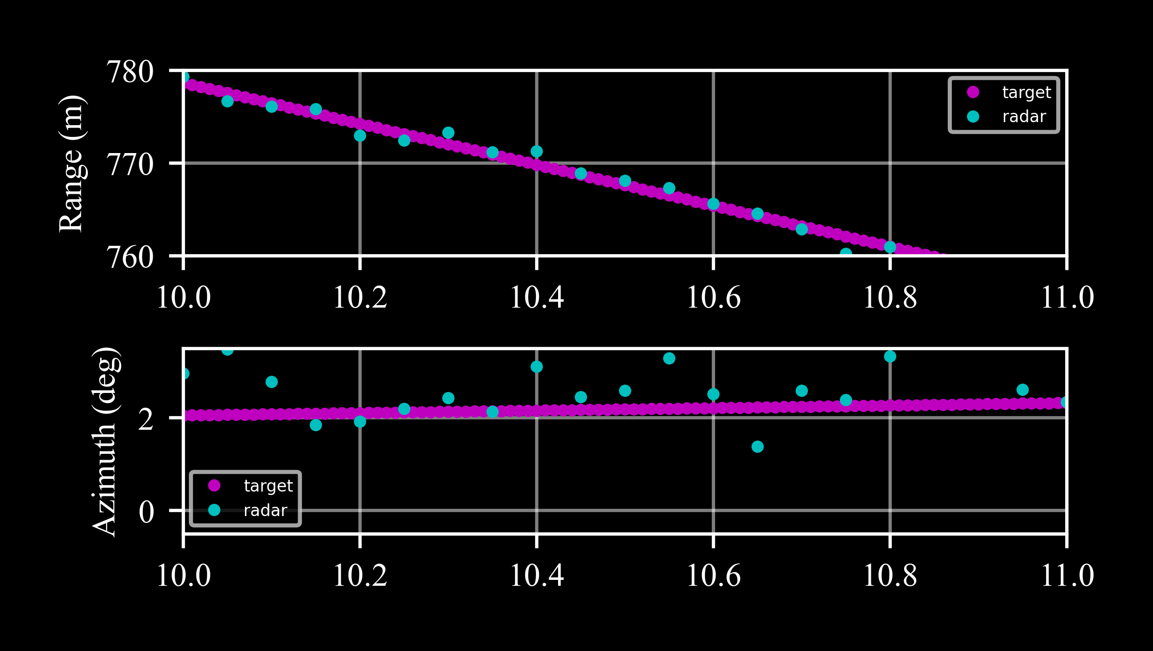
The sample rate of the radar was set by the parameter dt = 0.05. In cycles that don’t satisfy t < last_t + dt, measure returns None, as shown in a close-up view: