c4dynamics.states.lib.quatbody.quatbody.plot

quatbody.plot(var, scale=1, ax=None, filename=None, darkmode=True, **kwargs)

Draws plots of trajectories or variable evolution over time.

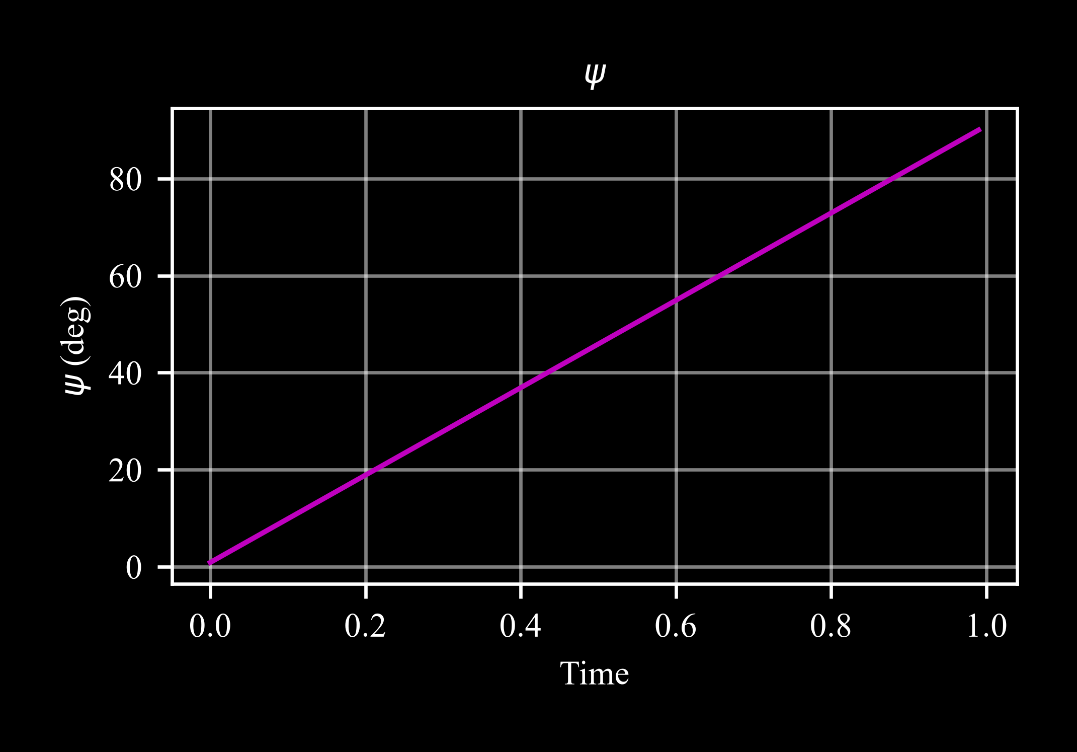
var can be each one of the state variables, the Euler angles phi, theta, psi, or top, side, for trajectories.

Parameters:

• var (str) – The variable to be plotted. Possible variables for trajectories: top, side. For time evolution, any one of the state variables is possible: x, y, z, vx, vy, vz, qw, qx, qy, qz, p, q, r, and the Euler angles phi, theta, psi (derived from the quaternion histories).

• scale (float or int, optional) – A scaling factor to apply to the variable values. Defaults to 1.

• ax (matplotlib.axes.Axes, optional) – An existing Matplotlib axis to plot on. If None, a new figure and axis will be created. By default None.

• filename (str, optional) – Full file name to save the plot image. If None, the plot will not be saved, by default None.

• darkmode (bool, optional) – Plot in a dark background style. By default True.

• **kwargs (dict, optional) – Additional key-value arguments passed to matplotlib.pyplot.plot. These can include any keyword arguments accepted by plot, such as color, linestyle, marker, etc.

Notes

• The method overrides the datapoint.plot.

• As in the rigidbody, Euler angles and angular rates are plotted in degrees and degrees per second, respectively.

• The quaternion components are plotted unitless.

Examples

>>> import c4dynamics as c4d
>>> import numpy as np

>>> dt = 0.01
>>> drone = c4d.quatbody(r = 90 * c4d.d2r)
>>> drone.I = [0.0082, 0.0082, 0.0149]
>>> for ti in np.arange(0, 1, dt):
...   drone.inteqm(np.zeros(3), np.zeros(3), dt)  
...   drone.store(ti)
>>> drone.plot('psi')