 ← Click to open in Google Colab
To download this notebook, click the download icon in the toolbar above and select the .ipynb format.
For any questions or comments, please open an issue on the c4dynamics issues page.
Neural Learning Control for Online Uncertain Dynamics Estimation#
First-principles models capture the main behavior of most engineered systems, but they are never exact. The gap between the model and reality comes from uncertain parameters, unmodeled nonlinear effects, coupling effects, and external disturbances. These factors limit the performance of purely model-based controllers.
This notebook presents a reusable framework for prototyping neural learning controllers that estimate these uncertainties online. Its emphasis is not the 2-DOF helicopter itself, but the environment abstraction, provided by c4dynamics, that separates the controller from the plant, allowing the same learning architecture to be evaluated on arbitrary nonlinear systems by replacing only the environment implementation.
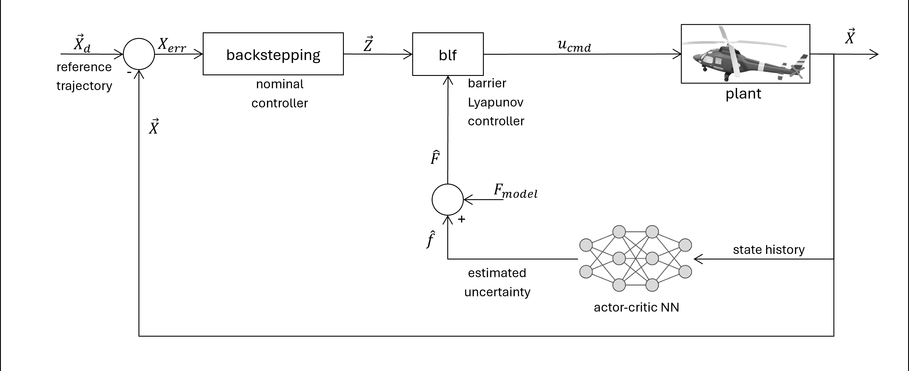
Figure 1: nonlinear controller with neural network uncertainty estimation.
Author#
This notebook was developed by Gilmar Tuta (@grep265) as part of the c4dynamics project, under the guidance of the c4dynamics maintainers.
Overview#
This notebook implements an adaptive control framework that combines a model-based backstepping controller with an actor–critic architecture for online uncertainty estimation. This differs from standard RL actor-critic where the actor outputs the control action. Here, the actor learns disturbance compensation while the critic provides adaptive gain modulation.
As shown in Figure 1, the desired trajectory \(X_d\) is compared with the system state \(X\). The resulting tracking error drives the backstepping controller, which computes the nominal control action from the available system model.
An Actor Network estimates the uncertain dynamics, \(\hat{f} = W_a^T H_a\), providing an adaptive compensation for modeling errors and external disturbances. The actor is trained online by gradient descent.
A Critic Network evaluates the quality of the actor’s compensation through a temporal-difference (\(TD\)) error, which is used to adapt the actor’s learning process.
Finally, a Barrier Lyapunov Function (\(BLF\)) incorporates state constraints into the control design, preventing the system from approaching predefined safety boundaries while preserving tracking performance.
Import required libraries
[1]:
import sys
# Check if Google Colab is running:
if "google.colab" in sys.modules:
    !pip install c4dynamics
[2]:
%matplotlib inline
import numpy as np
import matplotlib.pyplot as plt
from matplotlib.gridspec import GridSpec
from scipy.integrate import solve_ivp
import c4dynamics as c4d
1. Backstepping - Nominal Controller#
This algorithm is designed for systems whose state can be split into two parts:
where:
that is, \(X_1\) represents position-like variables, and \(X_2\) represents their corresponding velocities.
Such a structure naturally arises in second-order systems (e.g. mechanical systems), where the dynamics can be written in control-affine form:
This structure enables to handle position and velocity errors separately
Compute backstepping error signals and the virtual control \(\alpha\).
where:
\(X_1\): position-like state vector, containing the pitch and yaw angles
\(X_2\): velocity-like state vector, containing the pitch and yaw angular rates
\(X_d\): desired reference trajectory for \(X_1\)
\(\alpha\): virtual control that defines the desired value of \(X_2\)
\(Z_1\): position tracking-error vector between \(X_1\) and \(X_d\)
\(Z_2\): velocity tracking-error vector between \(X_2\) and \(\alpha\)
\(K_1\): positive backstepping gain matrix for the \(Z_1\) error
\(K_2\): positive backstepping gain matrix for the \(Z_2\) error
[3]:
def backstepping(x1: np.ndarray, x2: np.ndarray,
                 xd: np.ndarray, xd_d: np.ndarray,
                 xd_dd: np.ndarray, K1: np.ndarray):
    """Compute backstepping tracking errors and virtual-control derivative.

    Args:
        x1: Position-like state vector.
        x2: Velocity-like state vector.
        xd: Desired position-like reference vector.
        xd_d: First derivative of the desired reference vector.
        xd_dd: Second derivative of the desired reference vector.
        K1: Backstepping gain matrix for the x1 error.

    Returns:
        A tuple (z1, z2, alpha_d) containing the position error, velocity
        error, and virtual-control derivative.
    """

    z1      = x1 - xd
    alpha   = -K1 @ z1 + xd_d   #  compute desired velocity
    z2      = x2 - alpha
    alpha_d = -K1 @ (x2 - xd_d) + xd_dd

    return z1, z2, alpha_d
2. Barrier Lyapunov Controller (BLF)#
where:
\(BLF\): barrier Lyapunov function term that grows as tracking errors approach their bounds
\(Z_{1}\): position tracking-error vector constrained by the barrier function
\(m\): number of constrained tracking-error components
\(k_b\): vector of barrier bounds for the components of \(Z_1\)
\(P\): regularized control allocation matrix \(GG^T + \omega I\)
\(G\): control-effectiveness matrix of the helicopter dynamics
\(\omega\): positive regularization coefficient used to keep \(P\) well conditioned
\(u\): control input vector applied to the helicopter
\(K_2\): positive backstepping gain matrix for the \(Z_2\) error
\(Z_2\): velocity tracking-error vector between \(X_2\) and the virtual control
\(F\): nonlinear dynamics vector of the helicopter model
\(\alpha_d\): time derivative of the virtual control \(\alpha\)
[4]:
def blf_control(z1: np.ndarray, z2: np.ndarray,
                    F: np.ndarray, G: np.ndarray,
                    alpha_d: np.ndarray,
                    K2: np.ndarray, omega: float,
                    kb: np.ndarray) -> np.ndarray:
    """ Compute the learning BLF control

    Args:
        z1: Position tracking-error vector.
        z2: Velocity tracking-error vector.
        F: Drift dynamics vector evaluated at the current state.
        G: Control-effectiveness matrix evaluated at the current state.
        alpha_d: Derivative of the virtual control from backstepping.
        K2: Backstepping gain matrix for the z2 error.
        omega: Regularization coefficient for the control solve matrix.
        kb: Barrier bounds for each z1 component.

    Returns:
        The two-element control input vector.
    """

    z1_safe  = np.clip(z1, -0.999 * kb, 0.999 * kb)
    blf = z1_safe / (kb**2 - z1_safe**2)

    P   = G @ G.T + omega * np.eye(2)
    rhs = -blf - K2 @ z2 - F + alpha_d

    return np.clip(G.T @ np.linalg.solve(P, rhs), -50.0, 50.0)
Controller Parameters#
Parameter |
Description |
|---|---|
\(K_1\) |
Position error gain |
\(K_2\) |
Velocity error gain |
\(k_b\) |
BLF barrier bounds for \(\theta\), \(\psi\) errors |
\(\omega\) |
P-matrix regulariser |
[5]:
# Controller gains
K1    = np.diag([15.0, 5.0]) # Position error gain
K2    = np.diag([2.0, 1.5])  # Velocity error gain
kb    = np.array([0.5, 1.6]) # BLF barrier bounds for θ, ψ errors
omega = 0.01                  # P-matrix regulariser
3. Neural Network Uncertainty Estimation#
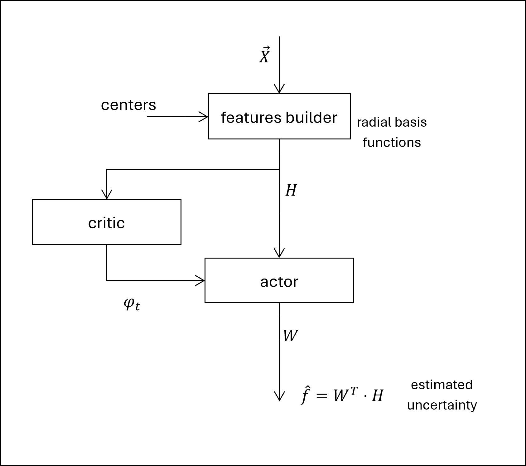
Figure 2: neural network architecture for uncertainty estimation.
Radial Basis Function Neural Networks (\(RBFNNs\))#
In this work, both the critic and actor use Radial Basis Function Neural Networks (\(RBFNNs\)) as linear-in-weights function approximators:
where:
\(f\): nonlinear function approximated by the RBF neural network
\(Z\): input vector to the RBF neural network
\(W\): neural-network weight vector used in the linear-in-weights approximation
\(H\): vector of RBF activations evaluated at \(Z\)
\(h\): individual Gaussian radial basis function activation
\(c\): RBF center location in the input space
\(b\): Gaussian width parameter that controls each basis function spread
\(m\): number of RBF nodes or basis functions
rbf_basis() computes the radial basis function activations \(𝐻(𝑍)\) for a given input vector \(𝑍\), set of centers \(𝑐_𝑖\), and Gaussian width \(𝑏\), enabling nonlinear function approximation through localized basis functions
[ ]:
def rbf_basis(Z: np.ndarray, centers: np.ndarray, width: float) -> np.ndarray:
    """Evaluate Gaussian radial basis functions at the input point.

    Args:
        Z: Input vector where the basis functions are evaluated.
        centers: RBF center locations, one center per row.
        width: Gaussian width parameter shared by all basis functions.

    Returns:
        A vector containing one RBF activation value per center.
    """

    diff = Z - centers
    return np.exp(-np.sum(diff**2, axis=1) / width**2)
make_centers() constructs a set of \(RBF\) centers \(c_i\) over the state/input domain, enabling localized Gaussian basis functions for accurate nonlinear function approximation
[ ]:
def make_centers(n_nodes: int, input_dim: int,
                 bounds: list, rng: np.random.Generator) -> np.ndarray:
    """Sample RBF centers uniformly within the provided bounds.

    Args:
        n_nodes: Number of RBF centers to generate.
        input_dim: Dimension of each center vector.
        bounds: Sequence of (min, max) bounds for each input dimension.
        rng: NumPy random number generator used for reproducible sampling.

    Returns:
        An array of shape (n_nodes, input_dim) containing sampled centers.
    """

    lo = np.array([b[0] for b in bounds])
    hi = np.array([b[1] for b in bounds])
    return rng.uniform(0, 1, size=(n_nodes, input_dim)) * (hi - lo) + lo
Critic#
The critic serves as the evaluator of the actor’s performance. Because the instantaneous cost \(I(t)\) is computed from the modeling residual \(e\) (which directly incorporates the actor’s compensation, the critic’s estimated value function \(\hat{J}(X)\) represents the expected long-term cumulative error under the current actor policy. As the actor’s compensation improves, the cost-to-go estimated by the critic decreases.
The instantaneous cost is the squared modeling residual evaluated after the actor’s learned compensation:
where:
\(e \in \mathbb{R}^n\): residual between the measured acceleration and the model’s prediction, with the actor’s current learned compensation subtracted
\(Q_e \succ 0\): positive-definite weighting on the residual (default: \(I_n\))
\(W_a^T H_a\): the actor’s current learned compensation
This cost has two key properties:
Bounded: as the actor learns to compensate the modeling error, \(e \to 0\) and the cost vanishes.
State-dependent: the mismatch is driven by physics (gravity, coupling), so the critic’s input \(X\) is the full state.
The value function is approximated by an RBF network:
The critic is updated using discrete-time \(TD\) (temporal difference):
The discount factor \(\gamma \in (0, 1)\).
\(Q_e\): residual cost matrix (default \(I_n\))
\(W_c\): critic neural-network weight vector
\(l_c\): critic learning rate
\(H_c\): critic basis-function activation vector
\(\hat{J}\): estimated long-term mismatch-to-go function
\(\gamma\): \(TD\) discount factor
\(dt\): integration time step
[ ]:
def critic_update(Wc: np.ndarray,
                     Hc: np.ndarray,
                     Hc_next: np.ndarray,
                     residual: np.ndarray,
                     Qe: np.ndarray,
                     gamma: float,
                     lc: float,
                     dt: float,
                     weight_limit: float | None = None):
    """Update critic weights with discrete-time TD (termporal difference) on the modeling mismatch.

    The critic estimates the long-term integrated mismatch I = e^T Q_e e
    under the current actor. With J_hat = Wc @ Hc and
    J_next = Wc @ Hc_next, the TD residual is
    phi = I*dt + gamma * (J_next - J_hat). The normalized update keeps the
    step size stable even when Hc activations vary.

    Args:
        Wc: Current critic weight vector, shape (Nc,).
        Hc: Critic RBF activation vector at state X_t.
        Hc_next: Critic RBF activation vector at state X_{t+1}.
        residual: Instantaneous modeling residual x2_dot_meas - (F + Gu) - W_a^T H_a.
        Qe: Residual cost matrix.
        gamma: TD discount factor.
        lc: Critic learning rate.
        dt: Integration time step.
        weight_limit: Optional critic-weight clipping bound.

    Returns:
        (Wc, J_hat, phi, I) after the critic update.
    """

    e  = residual
    I  = e @ Qe @ e
    J  = Wc @ Hc
    Jn = Wc @ Hc_next
    phi = I * dt + gamma * (Jn - J)

    norm = 1.0 + Hc @ Hc
    Wc = Wc + lc * phi * Hc / norm * dt

    if weight_limit is not None:
        Wc = np.clip(Wc, -weight_limit, weight_limit)

    J_hat = max(0.0, J)

    return Wc, J_hat, phi
Actor#
The actor network is responsible for evaluating the known dynamics. The actor here is updated directly using the gradient of the instantaneous modeling residual cost (\(2 \cdot Q_e \cdot e\)). The critic’s role is to modulate the step size of this update using its \(TD\) (temporal difference) error (\(\phi\)), scaling up the update rate when performance is unexpectedly good, and scaling it down when performance is unexpectedly poor.
The actor weights are updated via a gradient descent step on the instantaneous modeling cost, with the step size adaptively modulated by the critic’s \(TD\) error:
The cost gradient is \({\partial I \over \partial (W_a^T H_a)} = -2 \cdot Q_e \cdot e\) as \(I = e^T \cdot Q_e \cdot e\). The critic-modulation gate \(g(\phi)\) reacts to the \(TD\) error:
When \(\phi > 0\) (the realized mismatch was larger than the critic predicted), \(\tanh(-\phi) < 0\) and the gate shrinks.
When \(\phi < 0\) (the actor did better than expected), the gate grows, pushing the actor harder in the same direction.
The gain \(\kappa \ge 0\) controls the critic’s influence on the actor. The residual \(e\) appears as the cost gradient of the value function, with the critic’s \(TD\) error providing the adaptive gain. A weight-decay term \(-\sigma \cdot W_a\) is added to the update to prevent unbounded growth.
where:
\(W_a\): actor neural-network weight matrix
\(l_a\): actor learning rate
\(H_a\): actor basis-function activation vector
\(e\): modeling residual
\(Q_e\): residual cost matrix
\(\phi\): critic \(TD\) residual
\(\hat{J}\): critic’s long-term mismatch-to-go estimate
\(\kappa\): critic-modulation gain
\(\sigma\): weight decay term
[ ]:
def actor_update(Wa: np.ndarray,
                     Ha: np.ndarray,
                     residual: np.ndarray,
                     Qe: np.ndarray,
                     phi: float,
                     la: float,
                     kappa: float,
                     dt: float,
                     weight_limit: float | None = None):
    """Update actor weights via a gradient descent step on the instantaneous modeling cost, critic-modulated.

    The cost gradient -2 Q_e e provides the descent direction;
    gradient descent subtracts it, so the update adds 2 Q_e e. The critic's TD
    error phi modulates the learning-rate gain so the actor pushes harder
    when the realized cost exceeded the critic's expectation.

    Args:
        Wa: Current actor weight matrix.
        Ha: Actor RBF activation vector.
        residual: Instantaneous modeling residual x2_dot_meas - (F + Gu) - W_a^T H_a.
        Qe: Residual cost matrix.
        phi: Critic TD residual (advantage-like signal).
        la: Actor learning rate.
        kappa: Critic modulation gain.
        dt: Integration time step.
        weight_limit: Optional actor-weight clipping bound.

    Returns:
        Updated actor weight matrix.
    """
    sigma = 0.01 # Small regularization term to prevent unbounded growth
    grad_imm = 2.0 * (Qe @ residual)
    gate     = 1.0 + kappa * np.tanh(-phi)
    dWa      = (
        la * gate * np.outer(Ha, grad_imm)
        - sigma * Wa
    )
    Wa       = Wa + dWa * dt

    if weight_limit is not None:
        Wa = np.clip(Wa, -weight_limit, weight_limit)

    return Wa
Neural Network Parameters#
Parameter |
Description |
|---|---|
\(l_c\) |
critic learning rate |
\(l_a\) |
actor learning rate |
\(b_c\) |
critic Gaussian width |
\(b_a\) |
actor Gaussian width |
\(N_c\) |
critic hidden nodes |
\(N_a\) |
actor hidden nodes |
\(\gamma\) |
discount factor |
\(Q_e\) |
residual cost matrix |
\(\kappa\) |
critic modulation gain on actor |
critic_bounds |
RBFNN critic centre bounds |
actor_bounds |
RBFNN actor centre bounds |
[ ]:
lc    = 5.0                    # critic learning rate
la    = 5.0                    # actor learning rate
bc    = 0.8                    # critic Gaussian width
ba    = 20.0                   # actor Gaussian width
Nc    = 32                     # critic hidden nodes
Na    = 64                     # actor hidden nodes
gamma = 0.999                  # discount factor: gamma = exp(-dt/tau) with tau ≈ 1 s; dt = 0.001 s, tau = 1 s => gamma = exp(-0.001/1) ≈ 0.999
Qe    = np.eye(2)              # residual cost weighting
kappa = 1.0                    # critic modulation gain on actor

# Safety bounds
Wc_max = 100.0                 # critic weight clipping bound
Wa_max = 100.0                 # actor weight clipping bound

# RBFNN center bounds
critic_bounds = [
    (-0.5, 0.5),
    (-1.6, 1.6),
    (-2.0, 2.0),
    (-2.0, 2.0)
]

actor_bounds = [
    (-0.3, 0.3),    # theta
    (-0.3, 0.3),    # psi
    (-1.0, 1.0),    # dot{theta}
    (-1.0, 1.0)    # dot{psi}
]
4. Plant Environment#
The objective of this project is not to provide a controller for a single helicopter model, but to provide a reusable environment for developing and evaluating learning-based controllers.
The controller interacts only with the environment through the system state and control inputs, allowing the plant implementation to be replaced without modifying the learning algorithm. This separation makes it possible to prototype different dynamic systems, inject modeling errors and disturbances, and compare control strategies under identical conditions.
The environment is responsible for
simulating the plant dynamics,
integrating the equations of motion,
defining reference trajectories,
introducing model uncertainties and disturbances,
providing observations to the controller, and
recording data for analysis and visualization.
Although this notebook demonstrates the framework using a 2-DOF helicopter, the same interface can be adapted to other nonlinear systems with minimal changes.
Custom Environment#
The controller assumes systems of the (control-affine) form:
where the full state vector is \(X = [X_1,\, X_2] \in \mathbb{R}^{2n}\), split into:
\(X_1 \in \mathbb{R}^n\): position-like state vector, such as positions or angles
\(X_2 \in \mathbb{R}^n\): velocity-like state vector, such as velocities or rates
and:
\(F(X) \in \mathbb{R}^n\): system internal dynamics
\(G(X) \in \mathbb{R}^{n \times m}\): control-input matrix
\(u \in \mathbb{R}^m\): control input vector
Here \(n\) is the number of generalized coordinates and \(m\) is the number of inputs. To plug in a new system into this controller, implement a class with these methods and information:
Input |
Output |
Description |
|
|---|---|---|---|
states |
None |
System states |
Defines the complete system state representation used by the controller. |
system parameters |
None |
Physical/model parameters |
Defines all model parameters required by the environment dynamics. |
F(X) |
X: full state vector |
Internal dynamics vector \(F(X)\) |
Computes the internal system dynamics excluding the control-input contribution. |
G(X) |
X: full state vector |
Control-input matrix \(G(X)\) |
Computes the input matrix mapping control inputs into the system dynamics. |
dynamics(t, X, u) |
t: simulation time, X: full state vector, u: control input vector |
Full state derivative \(\dot{X}\) |
Returns the complete nonlinear state equation used for numerical integration and simulation. |
reference(t) |
t: simulation time |
Desired trajectory \((x_d,\ \dot{x}_d,\ \ddot{x}_d)\) |
Provides the desired reference trajectory and its derivatives required by the controller. |
class MySystem(c4dynamics.state):

    # State variables
    var_1: float
    ...
    var_n: float

    dvar_1: float
    ...
    dvar_n: float


    # Define physical/model parameters
    parameter_1 = ...
    parameter_2 = ...
    ...

    def __init__(self, var_1=var_1_0, ..., dvar_1=dvar_1_0, ...):
        ''' Initialize state variables '''

    def F(self, X):
        ''' Internal dynamics '''
        return F

    def G(self, X):
        ''' Input matrix '''
        return G

    def dynamics(self, t, X, u):
        ''' Full state equation '''

        X1_dot = X2
        X2_dot = F(X) + G(X) @ u

        return [X1_dot, X2_dot]

    def reference(self, t):
        ''' Desired trajectory '''

        xd     = ...
        xd_dot = ...
        xd_ddot = ...

        return xd, xd_dot, xd_ddot

    def split(self, X=None):
        ''' Split state vector into position and velocity components '''

        x = self.X if X is None else X
        n = len(x) // 2
        return x[:n], x[n:]
To create a custom environment, define a class that inherits from c4dynamics.state and follows the structure of MySystem.
Helicopter Example#
System Dynamics#
The system under consideration is a laboratory-scale 2-DOF helicopter, which can rotate in pitch and yaw directions and is actuated by two independent DC motors generating thrust forces. The system exhibits strong nonlinear coupling between these two axes. These characteristics make the control problem particularly challenging, as the controller must handle nonlinearities, coupling effects, and incomplete knowledge of the system while maintaining stable and accurate trajectory tracking.
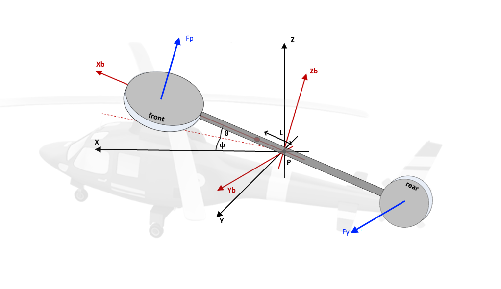
Figure 3: Helicopter diagram of a laboratory model mounted on a fixed base with two propellers driven by DC motors.
Clarifications for figure 3:
No translational motion exists
The front rotor generates thrust \(F_p\) and controls the pitch (\(\theta\)) motion
The rear rotor generates thrust \(F_y\) and controls the yaw (\(\psi\)) motion
The connecting beam is fixed at point \(P\) which is used as the origin of the coordiante systems
The helicopter center of mass is located at a distance \(L\) from point \(P\)
The inertial reference system (black) is fixed with origin at \(P\)
The body reference system (red) has an origin at \(P\) and rotates with the helicopter laboratory model
The azimuth angle \(\psi\) is the first rotation in the series and is given by a rotation about the \(Z\) inertial axis
The elevation angle \(\theta\) is the second rotation and is given by a rotation about the \(Y_b\) body axis
where:
\(\theta\): pitch angle
\(\psi\): yaw angle
\(\dot{\theta}\): pitch angular velocity
\(\dot{\psi}\): yaw angular velocity
\(V_p\): pitch motor input voltage
\(V_y\): yaw motor input voltage
\(D_p\): pitch viscous friction constant
\(D_y\): yaw viscous friction constant
\(J_p\): pitch-axis moment of inertia
\(J_y\): yaw-axis moment of inertia
\(K_{pp}\): torque thrust gain on the pitch axis from the pitch propeller
\(K_{py}\): torque thrust gain on the pitch axis from the yaw propeller
\(K_{yp}\): torque thrust gain on the yaw axis from the pitch propeller
\(K_{yy}\): torque thrust gain on the yaw axis from the yaw propeller
\(g\): gravitational acceleration
\(L_{cm}\): the center-of-mass distance from the body-fixed frame origin
\(M\): the helicopter’s mass
Dynamics clarifications:
Ideally, the front rotor would generate pure pitch motion and the rear rotor pure yaw motion.
In reality, the system is nonlinear because the pitch and yaw motions are dynamically coupled, as expressed in items (3) and (6).
The term in the left \((J_p + M \cdot L_{cm}^2) \cdot \ddot{\theta}\) is the rotational analogue of Newton’s second law \(m \cdot a\), where \((J_p + M \cdot L_{cm}^2)\) is the effective pitch-axis inertia and \(\ddot{\theta}\) is the pitch angular acceleration.
The term \(K_{pp} \cdot V_p\) represents the primary control action of the front rotor on the pitch axis, i.e. the pitch torque generated by the front motor voltage.
\(K_{py} \cdot V_y\) represents actuator coupling: an unintended contribution of the yaw rotor to the pitch dynamics due to non-ideal mechanics.
\(M \cdot g \cdot L_{cm} \cdot \cos\theta\) is the gravitational restoring torque acting on a rigid body.
\(D_p \cdot \dot{\theta}\) models viscous rotational damping opposing the pitch angular velocity.
The term \(M \cdot L_{cm}^2 \cdot \dot{\psi}^2 \cdot \sin\theta \cdot \cos\theta\) is a major coupling term. It originates from centrifugal inertial effects caused by the simultaneous yaw rotation and pitch orientation of the rigid body. As the helicopter rotates in yaw, the center of mass follows a curved trajectory around the yaw axis, generating additional apparent torques that couple the yaw motion into the pitch dynamics.
The terms in the yaw equation follow the same structure, besides \(2 \cdot M \cdot L_{cm}^2 \cdot \dot{\psi} \cdot \dot{\theta} \cdot \sin(\theta) \cdot \cos(\theta)\) which is the second major coupling term. It originates from the Coriolis-like inertial effects caused by the simultaneous pitch and yaw rotational motion of the rigid body. The interaction between the angular velocities generates additional apparent torques that couple the pitch motion into the yaw dynamics.
The state variables are defined as
For this example, \(n = 2\) (pitch and yaw) and \(m = 2\) (pitch motor voltage, yaw motor voltage), therefore:
and
Define initial states
[11]:
theta0 = 0.0  # [rad]
psi0 = 0.0  # [rad]
thetadot0 = 0.0  # [rad/s]
psidot0 = 0.0  # [rad/s]
Following the formulation
the helicopter dynamics are implemented through the functions F(X) and G(X) in environments.py.
Import environment
[12]:
from c4dynamics.envs.environments import helicopter

env = helicopter(theta=theta0, psi=psi0, dtheta=thetadot0, dpsi=psidot0)
print(env)
print(env.X)
[ θ  ψ  dtheta  dpsi ]
[0. 0. 0. 0.]
Dynamics Mismatch#
The gap between the controller’s model and the true plant is simulated by intentionally adding a mismatch to the physical parameters that appear in F(X) and G(X). Two categories of uncertainty are introduced:
Inertia uncertainty: the mass M, pitch inertia Jp, and yaw inertia Jy. This represents changes in the center of mass, inaccuracies in CAD modelling, and errors in inertia identification.
Aerodynamic gain uncertainty: the thrust gains Kpy (pitch from yaw rotor) and Kyy (yaw from yaw rotor). This represents imprecise motor/propeller models and errors in thrust coefficient identification.
The plant dynamics uses F(X) and G(X) with the nominal parameters, while the controller uses the perturbed parameter values. The resulting residual is the signal the actor-critic learns to cancel, and its magnitude depends directly on the size of these parameter mismatches:
The parameter mismatches were chosen to be large enough to challenge the nominal backstepping controller, thereby creating a meaningful residual for the actor–critic component to learn and compensate.
[13]:
mass_factor = 1.2
jy_factor   = 0.2
jp_factor   = 0.1
kpy_factor  = 1.35
kyy_factor  = 0.4
Desired Setpoint#
The desired trajectory used in this study consists of smooth sinusoidal functions for both pitch and yaw angles, which are commonly used in control system validation. This type of trajectory is particularly suitable because it continuously excites the system dynamics, allowing the controller’s performance to be evaluated under varying conditions rather than at a single operating point.
You can find the reference trajectory implementation for the helicopter example in the reference() method of environments.py.
5. Simulation#
For each step:
Log data for analysis
Evaluate updated system model
Get reference trajectory
Compute backstepping errors
Compute Lyapunov control
Integrate the TRUE dynamics
Evaluate critic features
Evaluate actor features
Evaluate the uncertainty
[ ]:
u_hist      = []
J_hat_hist  = []
u_k2_hist   = []
u_F_hist    = []
phi_hist    = []
residual_hist = []

seed = 42

# RBFNN centre placement
rng = np.random.default_rng(seed)

# Critic input: Zc = X (full states)
critic_centers = make_centers(Nc, 4, critic_bounds, rng)

# Actor input: Za = X (full states)
actor_centers  = make_centers(Na, 4, actor_bounds, rng)


def run_controller(dt: float = 0.001, T: float = 25.0, learning: bool = True):
    """ Run the helicopter simulation over the requested horizon.

    Args:
        dt: Simulation integration time step, in seconds.
        T: Total simulation duration, in seconds.
        seed: Random seed used to generate RBF centers.
        learning: Whether to use learned control input.

    Returns:
        None. The function updates the global env state history and
        appends control inputs to u_hist.
    """

    # Clear history from previous runs
    u_hist.clear()
    J_hat_hist.clear()
    phi_hist.clear()
    residual_hist.clear()
    env.reset()
    env.X = env.X0.copy()

    # Weight initialisation
    Wc = np.random.default_rng(seed).normal(0, 0.01, size=Nc)
    Wa = np.random.default_rng(seed).normal(0, 0.01, size=(Na, 2))

    Hc_prev = np.zeros(Nc)
    u  = np.zeros(2)
    f_hat  = np.zeros(2)
    J_hat = 0.0
    phi_td = 0.0
    residual = np.zeros(2)


    for t in np.arange(0, T, dt):

        env.store(t)
        u_hist.append(u.copy())
        J_hat_hist.append(J_hat)
        phi_hist.append(phi_td)
        residual_hist.append(np.linalg.norm(residual))

        # Model with intentionally perturbed parameters (uncertainty)
        F_control = env.F(mass = env.M * mass_factor, jy = env.Jy * jy_factor, jp = env.Jp * jp_factor)
        G_control = env.G(mass = env.M * mass_factor, jy =  env.Jy * jy_factor, jp = env.Jp * jp_factor,
                          kpy = env.Kpy * kpy_factor, kyy = env.Kyy * kyy_factor)

        # Reference trajectory
        xd, xd_d, xd_dd = env.reference(t)
        x1, x2 = env.split(env.X.copy())

        # Backstepping error variables
        z1, z2, alpha_d = backstepping(x1, x2, xd, xd_d, xd_dd, K1)


        # Compute control signal using RLC_BLF control law
        F = F_control + f_hat

        u = blf_control(
            z1, z2, F, G_control, alpha_d, K2, omega, kb
        )

        # Integrate ODE
        sol_env = solve_ivp(
            env.dynamics,
            [t, t + dt],
            env.X,
            args=(u,),
            method='RK45',
            max_step=dt,
            rtol=1e-6,
            atol=1e-9
        )
        env.X = sol_env.y[:, -1]

        # Measured acceleration residual
        _, x2_update  = env.split(env.X)
        x2_dot_meas = (x2_update - x2) / dt
        residual = (
            x2_dot_meas
            - F_control
            - G_control @ u
            - f_hat
        )

        # Actor - critic

        # Critic NN
        Hc = rbf_basis(env.X, critic_centers, bc)
        # Critic update - produces phi for the actor's gain modulation
        Wc, J_hat, phi_td = critic_update(
            Wc, Hc_prev, Hc, residual, Qe, gamma, lc, dt,
            weight_limit=Wc_max,
        )
        # features at next state
        Hc_prev = Hc.copy()

        # Neural Network Compensation
        Ha = rbf_basis(env.X, actor_centers, ba)
        Wa = actor_update(
            Wa, Ha, residual, Qe, phi_td, la, kappa, dt,
            weight_limit=Wa_max,
        )
        f_hat = np.clip(Wa.T @ Ha, -20.0, 20.0) * learning
6. Results#
Plotting Functions#
[ ]:
def plot_state_comparison(t_hist, theta_disabled, psi_disabled,
                          theta_enabled, psi_enabled, env):
    """Plot learning-enabled vs learning-disabled state outputs.

    Args:
        t_hist: Time array from simulation.
        theta_disabled: Pitch angle history (learning disabled).
        psi_disabled: Yaw angle history (learning disabled).
        theta_enabled: Pitch angle history (learning enabled).
        psi_enabled: Yaw angle history (learning enabled).
        env: Environment object for computing desired trajectory.
    """
    # Compute desired trajectory
    theta_d = np.array([env.reference(ti)[0][0] for ti in t_hist])
    psi_d   = np.array([env.reference(ti)[0][1] for ti in t_hist])

    fig = plt.figure(figsize=(10, 8))
    fig.suptitle('State Outputs', fontsize=12, fontweight='bold')
    gs = GridSpec(2, 1, hspace=0.45)

    ax = fig.add_subplot(gs[0])
    ax.plot(t_hist, theta_d * c4d.r2d,        'k--', lw=1.5, label='desired')
    ax.plot(t_hist, theta_disabled * c4d.r2d, 'r-',  lw=1.0, label='learning disabled')
    ax.plot(t_hist, theta_enabled * c4d.r2d,  'lime', lw=1.0, label='learning enabled')
    ax.legend(fontsize=8, loc='upper right')
    c4d.plotdefaults(ax, title=r'$\theta$', xlabel='', ylabel='Pitch (deg)')

    ax = fig.add_subplot(gs[1])
    ax.plot(t_hist, psi_d * c4d.r2d,        'k--', lw=1.5, label='desired')
    ax.plot(t_hist, psi_disabled * c4d.r2d, 'r-',  lw=1.0, label='learning disabled')
    ax.plot(t_hist, psi_enabled * c4d.r2d,  'lime', lw=1.0, label='learning enabled')
    ax.legend(fontsize=8, loc='upper right')
    c4d.plotdefaults(ax, title=r'$\psi$', xlabel='Time (s)', ylabel='Yaw (deg)')

    plt.show()


def plot_input_comparison(t_hist, u_disabled, u_enabled):
    """Plot learning-enabled vs learning-disabled control inputs.

    Args:
        t_hist: Time array from simulation.
        u_disabled: Control input array (learning disabled), shape (N, 2).
        u_enabled: Control input array (learning enabled), shape (N, 2).
    """
    def _style(ax, ylabel='', title=''):
        ax.set_xlabel('Time (s)', fontsize=9)
        ax.set_ylabel(ylabel,     fontsize=9)
        ax.set_title(title,       fontsize=10, fontweight='bold')
        ax.set_xlim(0, 25)
        ax.grid(True, linestyle='--', linewidth=0.4, alpha=0.6)
        ax.tick_params(labelsize=8)
        ax.legend(fontsize=8, loc='upper right')

    fig = plt.figure(figsize=(10, 5))
    fig.suptitle('Control Inputs', fontsize=12, fontweight='bold')
    gs = GridSpec(1, 2, hspace=0.35, wspace=0.35)

    Vpitch_dis, Vyas_dis = u_disabled.T
    Vpitch_en,  Vyas_en  = u_enabled.T

    ax = fig.add_subplot(gs[0])
    ax.plot(t_hist, Vpitch_dis, 'r-',   lw=1.0, label='disabled')
    ax.plot(t_hist, Vpitch_en,  'lime', lw=1.0, label='enabled')
    _style(ax, ylabel='Voltage [V]', title=r'$u_1$ (Pitch)')

    ax = fig.add_subplot(gs[1])
    ax.plot(t_hist, Vyas_dis, 'r-',   lw=1.0, label='disabled')
    ax.plot(t_hist, Vyas_en,  'lime', lw=1.0, label='enabled')
    _style(ax, ylabel='Voltage [V]', title=r'$u_2$ (Yaw)')

    plt.show()


def plot_critic_comparison(t_hist, J_hat_disabled, phi_disabled, residual_disabled,
                           J_hat_enabled, phi_enabled, residual_enabled):
    """Plot learning-enabled vs learning-disabled critic and cost signals.

    Args:
        t_hist: Time array from simulation.
        J_hat_disabled: Critic estimated mismatch-to-go (learning disabled).
        phi_disabled: TD (temporal difference) residual (learning disabled).
        residual_disabled: Modeling residual norm (learning disabled).
        J_hat_enabled: Critic estimated mismatch-to-go (learning enabled).
        phi_enabled: TD residual (learning enabled).
        residual_enabled: Modeling residual norm (learning enabled).
    """
    def _style(ax, ylabel='', title=''):
        ax.set_xlabel('Time (s)', fontsize=9)
        ax.set_ylabel(ylabel,     fontsize=9)
        ax.set_title(title,       fontsize=10, fontweight='bold')
        ax.set_xlim(0, 25)
        ax.grid(True, linestyle='--', linewidth=0.4, alpha=0.6)
        ax.tick_params(labelsize=8)
        ax.legend(fontsize=8, loc='upper right')

    fig = plt.figure(figsize=(10, 8))
    fig.suptitle('Critic and Cost', fontsize=12, fontweight='bold')
    gs = GridSpec(3, 1, hspace=0.45)

    ax = fig.add_subplot(gs[0])
    ax.plot(t_hist, J_hat_disabled, 'r-',   lw=1.0, label='disabled')
    ax.plot(t_hist, J_hat_enabled,  'lime', lw=1.0, label='enabled')
    _style(ax, title=r'Critic estimated mismatch-to-go $\hat{J}$')

    ax = fig.add_subplot(gs[1])
    ax.plot(t_hist, phi_disabled, 'r-',   lw=1.0, label='disabled')
    ax.plot(t_hist, phi_enabled,  'lime', lw=1.0, label='enabled')
    _style(ax, title=r'TD Residual $\phi$')

    ax = fig.add_subplot(gs[2])
    ax.plot(t_hist, residual_disabled, 'r-',   lw=1.0, label='disabled')
    ax.plot(t_hist, residual_enabled,  'lime', lw=1.0, label='enabled')
    _style(ax, title=r'Modeling residual norm $\|e\|$')

    plt.show()
Comparison: Learning Enabled vs Disabled#
[16]:
DT = 0.001    # integration step [s]
T  = 25.0     # simulation duration [s]

# Learning disabled
run_controller(dt = DT, T = T, learning = False)
t_hist, theta_dis = env.data('theta')
_,       psi_dis  = env.data('psi')
u_dis          = np.array(u_hist)
J_hat_dis      = np.array(J_hat_hist)
phi_dis        = np.array(phi_hist)
residual_dis   = np.array(residual_hist)

# Learning enabled
run_controller(dt = DT, T = T, learning = True)
_, theta_en = env.data('theta')
_, psi_en   = env.data('psi')
u_en          = np.array(u_hist)
J_hat_en      = np.array(J_hat_hist)
phi_en        = np.array(phi_hist)
residual_en   = np.array(residual_hist)
State Outputs#
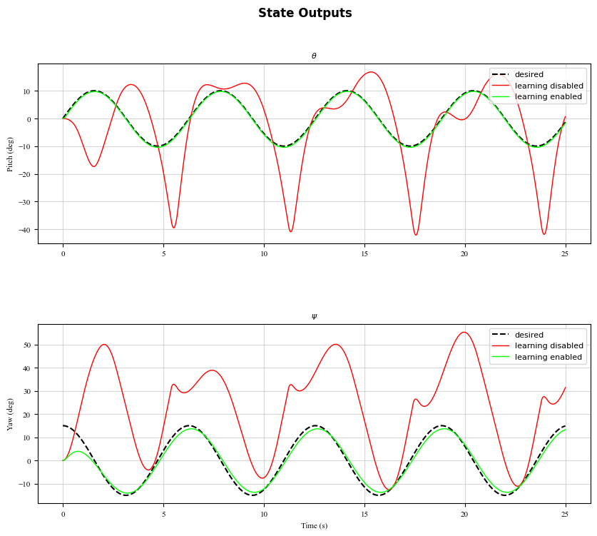
The following plots compare the closed-loop response of the controller under two conditions: learning disabled and learning enabled, both against the desired reference trajectory. With learning disabled, the nominal controller relies entirely on the mismatched model, resulting in persistent tracking errors. Enabling the actor-critic compensation reduces these errors, confirming that the learned component effectively addresses the modeling gap.
[17]:
plot_state_comparison(t_hist, theta_dis, psi_dis, theta_en, psi_en, env)
Control Inputs#
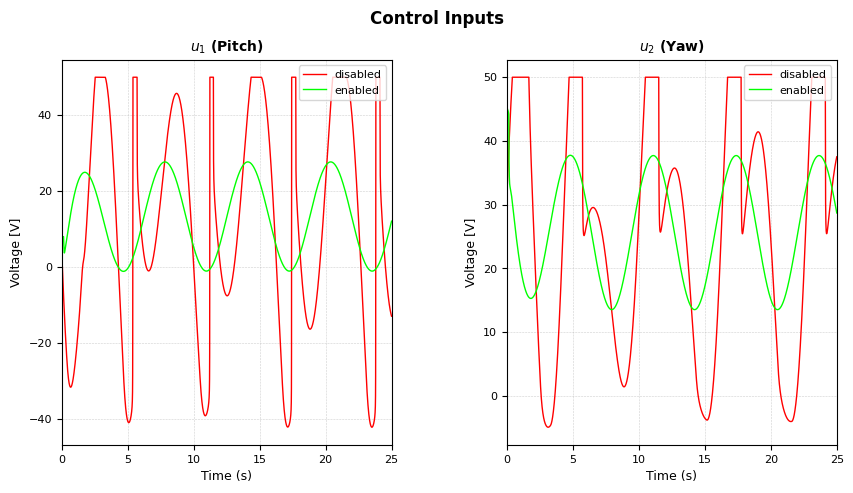
The control input comparison shows how the total control effort changes between the two configurations. With learning enabled, the actor’s learned compensation \(u_{\text{learned}}\) partially offsets the modeling mismatch, allowing the model-based component \(u_{\text{model}}\) to bridge the gap between the nominal model and the true plant dynamics. The resulting total control signals differ in both magnitude and waveform, reflecting the redistribution of effort between the model-based and learning-based components.
[18]:
plot_input_comparison(t_hist, u_dis, u_en)
Critic and Cost#
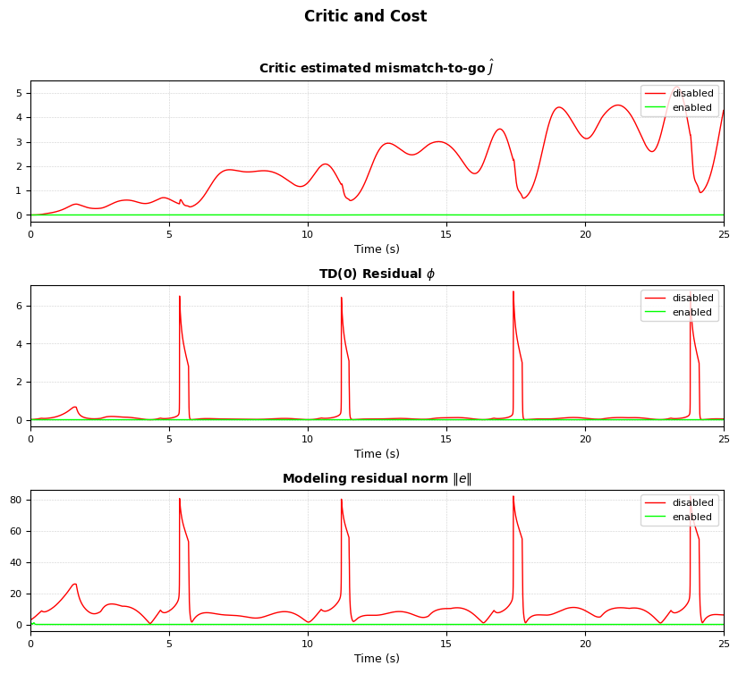
Three internal signals are compared to illustrate the learning dynamics: the critic’s estimated mismatch-to-go \(\hat{J}\), the \(TD\) (temporal difference) residual \(\phi\), and the instantaneous modeling residual norm \(\|e\|\). The residual norm directly measures how well the actor compensates for the modeling gap. The critic’s value estimate \(\hat{J}\) reflects the expected long-term cumulative cost under the current actor policy, while \(\phi\) indicates whether the realized cost exceeded or fell below the critic’s prediction at each step.
[19]:
plot_critic_comparison(t_hist, J_hat_dis, phi_dis, residual_dis,
                       J_hat_en, phi_en, residual_en)
RBF Trajectories#
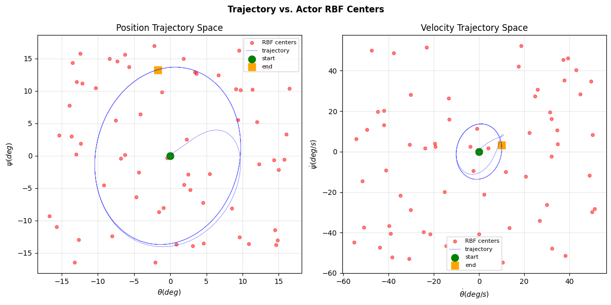
The trajectory comparison shows the state trajectory projected into the actor’s RBF input space, overlaid on the learned center locations. The left subplot displays the position trajectory in \((\theta, \psi)\), while the right subplot shows the velocity trajectory in \((\dot{\theta}, \dot{\psi})\). The coverage of the trajectory relative to the RBF centers indicates how well the actor’s basis functions span the regions visited during operation, ensuring that the learned compensation is effectively represented across the operating envelope.
[20]:
# Trajectory in actor RBF input space vs. center locations
# Actor input: [z1_theta, z1_psi, z2_theta, z2_psi]

if actor_centers.shape[1] == 4:
    fig, axes = plt.subplots(1, 2, figsize=(12, 6))
else:
    fig, axes = plt.subplots(1, 2, figsize=(12, 6))

fig.suptitle('Trajectory vs. Actor RBF Centers', fontsize=12, fontweight='bold')

# Extract trajectory
traj_z1_theta   = env.data('theta', scale = c4d.r2d)[1]
traj_z1_psi     = env.data('psi', scale = c4d.r2d)[1]
traj_z2_theta   = env.data('dtheta', scale = c4d.r2d)[1]
traj_z2_psi     = env.data('dpsi', scale = c4d.r2d)[1]

# Plot 1: z1 (position error) space
ax = axes[0]

ax.scatter(actor_centers[:, 0] * c4d.r2d, actor_centers[:, 1] * c4d.r2d, c='red', s=ba, alpha=0.5, label='RBF centers')
ax.plot(traj_z1_theta, traj_z1_psi, 'b-', linewidth=0.5, alpha=0.6, label='trajectory')
ax.scatter(traj_z1_theta[0], traj_z1_psi[0], c='green', s=100, marker='o', label='start')
ax.scatter(traj_z1_theta[-1], traj_z1_psi[-1], c='orange', s=100, marker='s', label='end')
ax.set_xlabel(r'$\theta (deg)$')
ax.set_ylabel(r'$\psi (deg)$')
ax.set_title('Position Trajectory Space')
ax.grid(True, alpha=0.3)
ax.legend(fontsize=8)
# ax.set_xlim(rbf_bounds[0])
# ax.set_ylim(rbf_bounds[1])

# Plot 2: z2 (velocity error) space
ax = axes[1]
ax.scatter(actor_centers[:, 2] * c4d.r2d, actor_centers[:, 3] * c4d.r2d, c='red', s=ba, alpha=0.5, label='RBF centers')
ax.plot(traj_z2_theta, traj_z2_psi, 'b-', linewidth=0.5, alpha=0.6, label='trajectory')
ax.scatter(traj_z2_theta[0], traj_z2_psi[0], c='green', s=100, marker='o', label='start')
ax.scatter(traj_z2_theta[-1], traj_z2_psi[-1], c='orange', s=100, marker='s', label='end')
ax.set_xlabel(r'$\dot{\theta} (deg/s)$')
ax.set_ylabel(r'$\dot{\psi} (deg/s)$')
ax.set_title('Velocity Trajectory Space')
ax.grid(True, alpha=0.3)
ax.legend(fontsize=8)

plt.tight_layout()
7. Summary#
This notebook presented a modular framework for developing adaptive learning controllers for nonlinear dynamical systems.
The controller combines
a backstepping baseline controller for guaranteed stabilization,
\(RBF\) neural networks to approximate unknown dynamics,
an actor network that learns the uncertainty compensation online, and
a critic that estimates the long-term cost.
The learning algorithm operates independently of the underlying plant through a dedicated environment, making it straightforward to replace the helicopter model with other nonlinear systems or to evaluate different uncertainty scenarios.
The simulation results demonstrate that enabling online learning substantially improves tracking performance compared with the baseline controller alone, highlighting the effectiveness of adaptive uncertainty estimation for compensating modeling errors and external disturbances.
The implementation is intended primarily as a research and prototyping platform, providing a clear reference architecture for experimenting with adaptive control, reinforcement learning, and online function approximation before deployment to real hardware.
References#
[1] Zhao et al., “Reinforcement Learning Control for a 2-DOF Helicopter With State Constraints: Theory and Experiments” IEEE Trans. Autom. Sci. Eng., Vol. 21, No. 1, Jan 2024. DOI: 10.1109/TASE.2022.3215738
[2] Quanser Inc., “Quanser 2-DOF Helicopter Laboratory Manual,” Quanser Aerospace, Instructor Manual, 2011.
[3] Lavretsky, E., & Wise, K. A. (2013). Robust and adaptive control: With aerospace applications. Springer London. DOI: 10.1007/978-3-031-38314-4