c4dynamics.eqm.integrate.int6q

c4dynamics.eqm.integrate.int6q(qb: quatbody, forces: ndarray | list, moments: ndarray | list, dt: float, derivs_out: bool = False) → ndarray[tuple[Any, ...], dtype[float64]] | Tuple[ndarray[tuple[Any, ...], dtype[float64]], ndarray[tuple[Any, ...], dtype[float64]]]

A step integration of the equations of motion, quaternion attitude.

This method makes a numerical integration using the fourth-order Runge-Kutta method.

The integrated derivatives are of six dimensional motion with quaternion attitude kinematics as given by eqm6q.

The result is an integrated state in a single interval of time where the size of the step is determined by the parameter dt. At the end of the step, the quaternion is normalized to a unit quaternion to prevent numerical drift.

Parameters:

• qb (quatbody) – The quatbody which state vector is to be integrated.

• forces (numpy.array or list) – An external forces array acting on the body.

• moments (numpy.array or list) – An external moments array acting on the body.

• dt (float) – Time step for integration.

• derivs_out (bool, optional) – If true, returns the translational and angular accelerations of the last step.

Returns:

• X (numpy.float64) – An integrated state.

• dxdt4 (numpy.float64, optional) – The translational and angular accelerations \([dv_x, dv_y, dv_z, dp, dq, dr]\) of the last step. Returned if derivs_out is set to True.

Algorithm

The integration steps follow the Runge-Kutta method:

1. Compute k1 = f(ti, yi)

2. Compute k2 = f(ti + dt / 2, yi + dt * k1 / 2)

3. Compute k3 = f(ti + dt / 2, yi + dt * k2 / 2)

4. Compute k4 = f(ti + dt, yi + dt * k3)

5. Update yi = yi + dt / 6 * (k1 + 2 * k2 + 2 * k3 + k4)

6. Normalize the quaternion.

Examples

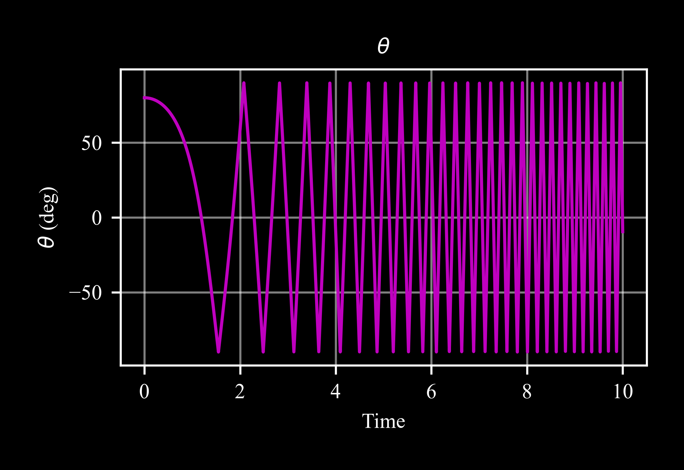
The equations of motion of a cylinderical body are integrated by using int6q.

Import required packages

>>> import c4dynamics as c4d
>>> import numpy as np

Settings and initial conditions

>>> dt = 0.5e-3
>>> t  = np.arange(0, 10, dt)
>>> theta0 =  80 * c4d.d2r       # deg
>>> Iyy    =  .4                 # kg * m^2
>>> length =  1                  # meter
>>> mass   =  0.5                # kg

Define the cylinderical-quatbody object

>>> qb = c4d.quatbody(theta = theta0)
>>> qb.I = [0, Iyy, 0]
>>> qb.mass = mass

Main loop:

>>> for ti in t:
...   qb.store(ti)
...   tau_g = -qb.mass * c4d.g_ms2 * length / 2 * c4d.cos(qb.theta)
...   qb.X = c4d.eqm.int6q(qb, np.zeros(3), [0, tau_g, 0], dt)

>>> qb.plot('theta')