• ← Click to open in Google Colab

• To download this notebook, click the download icon in the toolbar above and select the .ipynb format.

• For any questions or comments, please open an issue on the c4dynamics issues page.

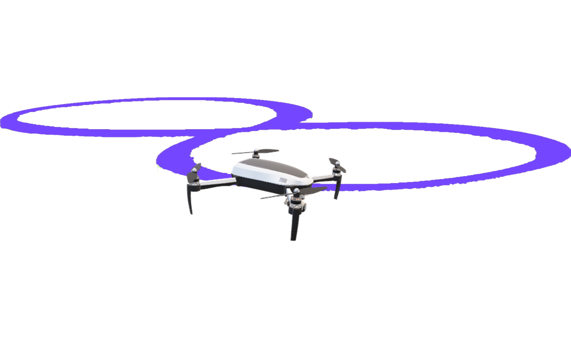
Quadcopter Cascade PID — Figure-8 Trajectory Tracking

This notebook presents a three-loop cascade PID simulation of a quadcopter tracking a figure-8 (\(\infty\)) trajectory. It models the quadcopter dynamics, builds the control hierarchy, and runs the simulation using c4dynamics.

---

Author

This notebook was developed by Usama Khan (@usama-k-mech) as part of the c4dynamics project, under the guidance of the c4dynamics maintainers.

Goal

Understand the following example and adjust it to simulate your drone parameters tracking figure-8.

---

Notebook Overview

1. Quadcopter initialization

2. Figure-8 dimensions setting

3. Cascade PID overview and architecture

4. Simulation

5. Results

• At the end of every section, a code snippet is configuring the simulating objects.

• After running the example, change the quadcopter and the figure-8 configurations to support your own system.

To keep the notebook focused on tuning and results, the implementation details are collected in a supporting utility file, ``quad_pid_utils.py``.

---

1. Setup

import sys
if 'google.colab' in sys.modules:
    !pip install c4dynamics

from urllib import request
request.urlretrieve('https://raw.githubusercontent.com/c4dynamics/c4dynamics/main/docs/source/programs/pid_cascade/quad_pid_utils.py', 'quad_pid_utils.py')

from quad_pid_utils import (run_fig8_pid,
                             plot_results,
                             compute_metrics
                             )

---

2. Quadcopter

State Variables

The quadcopter is a 12-state rigid body object with position, velocity, Euler angles, and body angular rates:

\[\mathbf{X} = [x,\ y,\ z,\ v_x,\ v_y,\ v_z,\ \varphi,\ \theta,\ \psi,\ p,\ q,\ r]^T\]

Where:

• \(x, y, z\): position of the quadcopter in the inertial frame [m]

• \(v_x, v_y, v_z\): linear velocity components in the inertial frame [m/s]

• \(\varphi\) (phi): roll angle — rotation about the body X-axis [rad]

• \(\theta\) (theta): pitch angle — rotation about the body Y-axis [rad]

• \(\psi\) (psi): yaw angle — rotation about the body Z-axis [rad]

• \(p, q, r\): angular rate components about the body X, Y, Z axes respectively [rad/s]

The four control inputs are:

\[\mathbf{U} = [F,\ \tau_\varphi,\ \tau_\theta,\ \tau_\psi]^T\]

Where:

• \(F\): total thrust force produced by all four rotors combined [N]

• \(\tau_\varphi\): roll torque — differential thrust between left and right motors [N·m]

• \(\tau_\theta\): pitch torque — differential thrust between front and rear motors [N·m]

• \(\tau_\psi\): yaw torque — differential drag torque from counter-rotating motor pairs [N·m]

The quadcopter starts on the ground stationary level. A quad object initializes the state, stores every sample during the simulation, and provides history retrieval for plotting and metrics via quad.data().

Reference Frame

In this work we adopt the FRD (front-right-down) for the body referece frame and ENU (east-north-up) for the inertial frame (see figure 1).

In this body frame convention, the thurst acts along the negative body z-axis (\(-z_b\)).

Positive rates about an axis is given by curling the right-hand fingers.

Propellers rotation:

Rotor 1: CCW (counter-clockwise)

Rotor 2: CCW

Rotor 3: CW

Rotor 4: CW

Yaw torque arises from the reaction torques of the rotors, with clockwise propeller causes a counter-clockwise moment on the quadcopter.

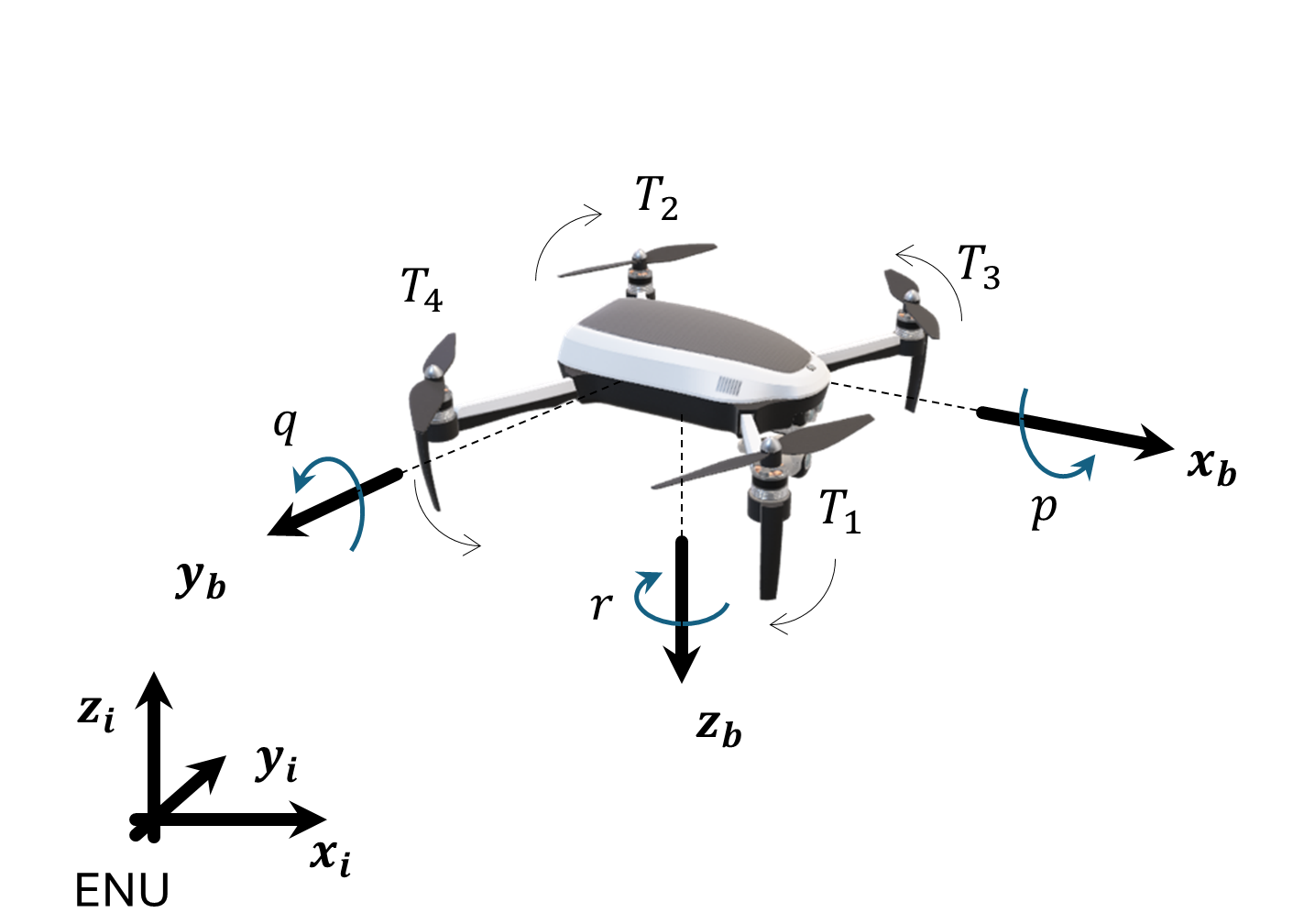
Figure 1: Reference systems. Inertial system: ENU (east, north, up). Body frame: (forward, right, down). Positive rotation about an axis is given by curling the right-hand fingers. Propellers rotation: 1: CCW (counter=clockwise) , 2: CCW, 3: CW, 4: CW.

Dynamics

The quadcopter is modeled by the full nonlinear Newton-Euler equations.

Translational dynamics (inertial frame):

\[m \ddot{\mathbf{r}} = \mathbf{F}_{thrust} + \mathbf{F}_{drag} + \mathbf{F}_{gravity}\]

Where:

• \(m\): total mass of the quadcopter [kg]

• \(\ddot{\mathbf{r}}\): linear acceleration vector in the inertial frame [m/s²]

• \(\mathbf{F}_{thrust}\): total rotor thrust force, projected from body frame to inertial frame [N]

• \(\mathbf{F}_{drag}\): aerodynamic drag force, proportional to velocity [N]

• \(\mathbf{F}_{gravity}\): gravitational force acting downward on the quadcopter [N]

The thrust \(F\) acts along \(-Z_b\) and is projected to the inertial frame via the ZYX rotation matrix.

Rotational dynamics (Euler’s equations in body frame):

\[\mathbf{I}\dot{\boldsymbol{\omega}} + \boldsymbol{\omega} \times \mathbf{I}\boldsymbol{\omega} = \boldsymbol{\tau}\]

Where:

• \(\mathbf{I}\): inertia tensor of the quadcopter body, diagonal with entries \(I_{xx}, I_{yy}, I_{zz}\) [kg·m²]

• \(\dot{\boldsymbol{\omega}}\): angular acceleration vector in the body frame [rad/s²]

• \(\boldsymbol{\omega} = [p, q, r]^T\): angular velocity vector in the body frame [rad/s]

• \(\boldsymbol{\omega} \times \mathbf{I}\boldsymbol{\omega}\): gyroscopic (Coriolis) term arising from the rotating body frame — couples the three rotation axes

• \(\boldsymbol{\tau} = [\tau_\varphi,\ \tau_\theta,\ \tau_\psi]^T\): torque vector produced by differential rotor thrust [N·m]. A gyroscopic coupling term from rotor angular momentum is also included.

The dynamics(t, y, quad, rotor_speeds) function computes the 12 state derivatives.

Integration is carried out by using scipy’s solve_ivp.

For the full theoretical background on rigid-body kinematics and the state representation used by c4dynamics, see the c4dynamics kinematics page.

Config

quadcopter = {
    'm'  : 0.468,      # mass [kg]
    'g'  : 9.81,       # gravity [m/s^2]
    'l'  : 0.225,      # arm length — center to motor [m]
    'kT' : 2.98e-6,    # thrust coefficient  [N/(rad/s)^2]
    'kQ' : 0.0382,     # torque coefficient  [N.m/(rad/s)^2]
    'Ixx': 4.856e-3,   # roll  inertia [kg.m^2]
    'Iyy': 4.856e-3,   # pitch inertia [kg.m^2]
    'Izz': 8.801e-3,   # yaw   inertia [kg.m^2]
    'Ax' : 0.30,       # aero drag — x
    'Ay' : 0.30,       # aero drag — y
    'Az' : 0.25,       # aero drag — z
    'Ar' : 0.20,       # rotational drag — angular rates
    'IR' : 3.357e-5,   # rotor inertia [kg.m^2]
}

---

3. Trajectory

The reference to the flight is a Lissajous figure-8 in the horizontal plane at a fixed altitude:

\[\begin{split}x_{ref}(t) = A \cdot \sin(\omega \cdot \tau) \\\end{split}\]

\[\begin{split}y_{ref}(t) = B \cdot \sin(2\omega \cdot \tau) \\\end{split}\]

\[z_{ref}(t) = z_{ref}\]

Where:

• \(x_{ref}, y_{ref}, z_{ref}\): desired position the quadcopter must track [m]

• \(A\): trajectory amplitude in the X direction [m]

• \(B\): trajectory amplitude in the Y direction [m]

• \(\omega\): angular frequency of the trajectory [rad/s]; period \(= 2\pi/\omega\)

• \(\tau = t - t_{takeoff}\): time elapsed since the figure-8 phase started [s]

• \(t_{takeoff}\): time at which the figure-8 phase begins [s]

This is a standard benchmark for trajectory tracking controllers because it combines simultaneous motion in both horizontal axes, continuous direction reversals, and a non-trivial curvature profile — all of which stress-test the controller’s ability to reject coupling errors and follow a dynamic reference.

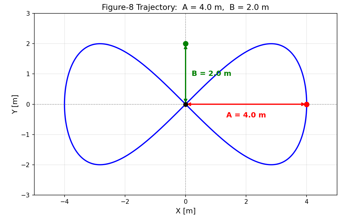
Figure 2: top view of a figure-8 trajectory with marks of the \(A\) and \(B\) dimensions.

Physical Meanings

Parameter	meaning
A	Half-width of the figure-8 in the X direction [m]. Larger values mean a wider trajectory.
B	Half-width in the Y direction [m]. Controls the “height” of each lobe of the figure-8.
omega	Angular frequency [rad/s]. Controls how fast the quadcopter flies the path. Period = \(2\pi/\omega\).
z_ref	Constant hover altitude [m]. The quadcopter holds this height throughout the maneuver.

3-Phase Flight

Phase	Duration	Description
Takeoff	0 — 8s	Z rises from 0 to z_ref on a smooth S-curve
Figure-8	8s — (end-8s)	X/Y track the Lissajous at constant altitude
Landing	last 8s	X/Y return to origin, Z descends to 0

• In the utility file quad_pid_utils.py, the functions position_reference(t, ...) and velocity_reference(t, ...) return the instantaneous reference position and velocity at any time t.

Config

trajectory = {
    'A'    : 4.0,    # figure-8 X amplitude [m]
    'B'    : 2.0,    # figure-8 Y amplitude [m]
    'omega': 0.1,    # angular frequency [rad/s]  (period ~ 62.8 s)
    'z_ref': 1.5,    # hover altitude [m]
    't_end': 90.0,   # total simulation time [s]
}

---

4. Cascade PID Control

Why Cascade PID?

A quadcopter is underactuated — 6 degrees of freedom, only 4 control inputs. To move horizontally the quadcopter must tilt, which means position and attitude are tightly coupled. A single PID loop cannot handle this. The cascade structure separates the problem by bandwidth:

Loop	Rate	Input	Output
Outer — Position	50 Hz	Position error \((x, y, z)\)	Desired angles \(\varphi_d, \theta_d\) + thrust \(F\)
Middle — Attitude	100 Hz	Angle error \((\varphi, \theta, \psi)\)	Desired body rates \((p_d, q_d, r_d)\)
Inner — Rate	200 Hz	Rate error \((p, q, r)\)	Torques \((\tau_\varphi, \tau_\theta, \tau_\psi)\)

Tuning order: always tune inner first, then middle, then outer. Each loop must be stable before the next loop is closed around it.

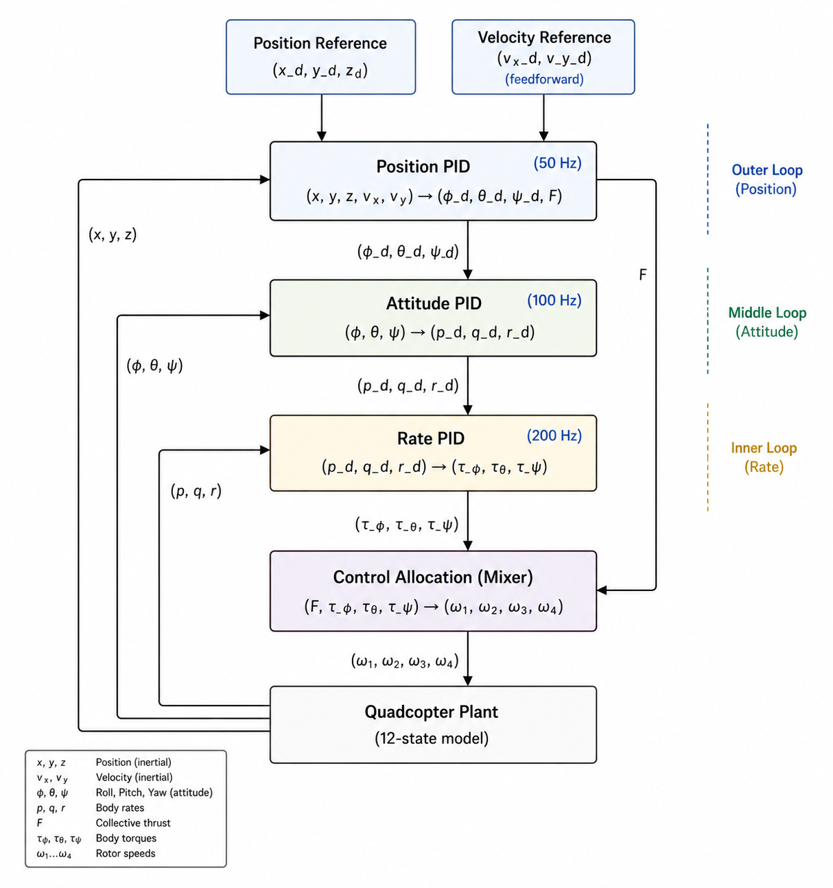
Figure 3: cascade PID with 3 loops - to control position (outer), attitude (middle), and rates (inner).

Control Law

Each controller implements:

\[u = K_p \cdot e + K_i \cdot \int e\, dt - K_d \cdot \dot{m}\]

Where:

• \(u\): control output — setpoint to the next inner loop, or actuator command for the innermost loop

• \(K_p, K_i, K_d\): proportional, integral, and derivative gains

• \(e\): error — difference between the desired setpoint and the current measured value

• \(\int e\, dt\): accumulated error over time

• \(\dot{m}\): time derivative of the measurement (not the error), to avoid derivative kick on setpoint changes

The derivative acts on the measurement \(\dot{m}\), not on the error — this eliminates derivative kick when the setpoint changes. All integrators include anti-windup clamping. The outer loop adds a velocity feedforward term to reduce phase lag on curved trajectories.

Control Allocation

The motor layout is (x) configuration.

The four control inputs \([F, \tau_\varphi, \tau_\theta, \tau_\psi]\) are mapped to individual rotor speeds by inverting the thrust-torque mixing matrix:

\[\begin{split}\begin{bmatrix} \Omega_1^2 \\ \Omega_2^2 \\ \Omega_3^2 \\ \Omega_4^2 \end{bmatrix} = \mathbf{\Gamma}^{-1} \begin{bmatrix} F \\ \tau_\varphi \\ \tau_\theta \\ \tau_\psi \end{bmatrix}\end{split}\]

Where:

• \(\Omega_1, \Omega_2, \Omega_3, \Omega_4\): individual rotor angular speeds [rad/s]

• \(\mathbf{\Gamma}^{-1}\): inverse of the thrust-torque mixing matrix — maps desired thrust and torques to individual rotor speeds

• \(F\): total desired thrust [N]

• \(\tau_\varphi, \tau_\theta, \tau_\psi\): desired roll, pitch, and yaw torques [N·m]

The normalized (geometric factors are handled separately) mixer matrix \(\mathbf{\Gamma}^{-1}\) for an x configuration with prepellents 1, 2 CCW and 3, 4 CW is given by:

\[\begin{split}\begin{bmatrix} 1 & -1 & \ \ \ 1 & \ \ \ 1 \\ 1 & \ \ \ 1 & -1 & \ \ \ 1 \\ 1 & \ \ \ 1 & \ \ \ 1 & -1 \\ 1 & -1 & -1 & -1 \end{bmatrix}\end{split}\]

This matrix is the inverse of the force–torque mapping derived from rotor positions and spin directions.

Each row corresponds to one motor, and each column represents the contribution of thrust, roll, pitch, and yaw.

The method allocate of ControlAllocator clamps \(\Omega_i^2 \geq 0\) (rotors cannot pull) and \(\Omega_i \leq \Omega_{max}\) before taking the square root.

Config

controller = {

    # Inner loop — angular rate (200 Hz)
    'Kp_p': 0.80,  'Ki_p': 0.0001,  'Kd_p': 0.010,
    'Kp_q': 0.80,  'Ki_q': 0.0001,  'Kd_q': 0.010,
    'Kp_r': 0.60,  'Ki_r': 0.0001,  'Kd_r': 0.008,

    # Middle loop — attitude (100 Hz)
    'Kp_phi'  : 6.0,  'Ki_phi'  : 0.0001,  'Kd_phi'  : 0.80,  'AW_phi'  : 0.5,
    'Kp_theta': 6.0,  'Ki_theta': 0.0001,  'Kd_theta': 0.80,  'AW_theta': 0.5,
    'Kp_psi'  : 4.0,  'Ki_psi'  : 0.5,     'Kd_psi'  : 0.40,  'AW_psi'  : 0.5,

    # Outer loop — position (50 Hz)
    'Kp_x': 0.80,  'Ki_x': 0.00,  'Kd_x': 0.50,  'AW_x': 0.5,
    'Kp_y': 1.00,  'Ki_y': 0.00,  'Kd_y': 0.70,  'AW_y': 0.5,
    'Kp_z': 10.0,  'Ki_z': 10.0,  'Kd_z': 1.50,  'AW_z': 3.0,

    # Velocity feedforward
    'Kff_x': 0.35,  'Kff_y': 0.40,

    # Limits
    'N_rate'        : 50,       # Filter coefficient for derivative term in rate controller
    'omega_max'     : 1000.0,   # max rotor speed [rad/s]
    'T_max_factor'  : 4,        # max thrust factor: T_max = T_max_factor * K_thrust * omega_max**2 [N]
    'T_min'         : 0.0,      # min thrust [N]
    'att_cmd_limit' : 0.314,    # Max attitude command [rad] = 18deg
    'yaw_rate_limit': 1.0,      # Max yaw rate command [rad/s]
}

---

5. Simulation

The simulation loop advances the quadcopter state from t = 0 to t = tf.

At each timestep the three cascade loops fire at their respective rates:

• the outer position loop every \(4\) steps (\(50 Hz\))

• the middle attitude loop every \(2\) steps (\(100 Hz\))

• the inner rate loop every step (\(200 Hz\)).

quad.store(t) logs the full state vector.

quad.storeparams(...) logs the control inputs.

After the loop, all histories are available via quad.data().

Config

simulation = {
    'dt': 5e-3,    # master timestep [s] = inner loop (200 Hz)
    'tf': 90.0,    # simulation end time [s]
}

Main Loop

# plug all the config files for the simulation entry:
config = {
    'quad': quadcopter,
    'controller': controller,
    'trajectory': trajectory,
    'sim': simulation
}

Run Simulation

quad = run_fig8_pid(config)

Simulation start  |  tf = 90.0 s  |  dt = 0.005 s
Simulation complete.

---

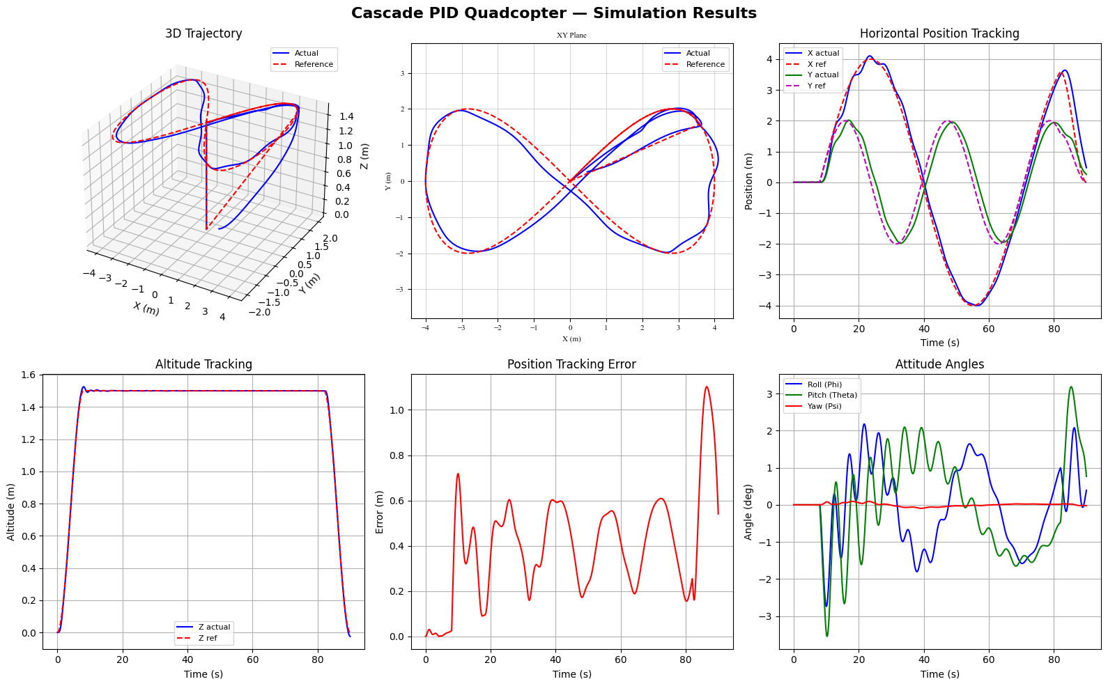
8. Results

What to Expect

A well-tuned cascade PID on this trajectory should show:

• Position — X and Y closely follow the sinusoidal references. Small amplitude and phase lag are normal.

• Altitude — Z rises sharply during takeoff, holds z_ref with very small deviation, and descends smoothly.

• Euler angles — roll and pitch stay within \(±15°\). Yaw remains near zero.

• 3D trajectory — a clean takeoff lobe, the figure-8 loops, and a straight descent to origin.

All plots are generated from quad.data() — the stored histories in the rigidbody object.

Trajectories and Angles

plot_results(quad, config['trajectory'])

Tracking Metrics

compute_metrics() computes RMSE for \(X, Y, Z\) tracking over the figure-8 phase only.

Normalized RMSE expresses tracking error as a percentage of trajectory amplitude.

Normalized RMSE	Interpretation
< 5%	Excellent
5 – 15%	Acceptable
> 15%	Retune from inner loop, or reduce omega

metrics = compute_metrics(quad, trajectory)

print('=' * 45)
print('   TRACKING PERFORMANCE METRICS')
print('=' * 45)
print(f'  RMSE x : {metrics["rmse_x"]:.4f} m  ({metrics["norm_x"]:.1f}% of X amplitude)')
print(f'  RMSE y : {metrics["rmse_y"]:.4f} m  ({metrics["norm_y"]:.1f}% of Y amplitude)')
print(f'  RMSE z : {metrics["rmse_z"]:.6f} m  ({metrics["norm_z"]:.3f}% of altitude)')
print(f'  Max altitude deviation : {metrics["max_z_dev"]*100:.2f} cm')
print('=' * 45)

=============================================
   TRACKING PERFORMANCE METRICS
=============================================
  RMSE x : 0.1992 m  (5.0% of X amplitude)
  RMSE y : 0.3831 m  (19.2% of Y amplitude)
  RMSE z : 0.002137 m  (0.142% of altitude)
  Max altitude deviation : 2.53 cm
=============================================