![]() ← Click to open in Google Colab
← Click to open in Google Colab
Interactive Guide to State Space and State Objects Modeling#
Welcome!
This notebook teaches the core workflow of c4dynamics through small, hands-on tasks. Each section asks you to run code, inspect results, and complete short exercises designed to build intuition.
Further Help and Documentation#
If you need clarification on any operation you encounter in this notebook, you can always refer to the State Objects page in the concepts section of the official documentation or to the State Class in the API section. You’ll find detailed explanations, examples, and the full specification of the state-object mechanism used throughout c4dynamics.
Setup#
[ ]:
# !pip install c4dynamics
Import necessary libraries:
[ ]:
import c4dynamics as c4d
import matplotlib.pyplot as plt
import numpy as np

# Sanity check: Print version
print("c4dynamics version:", c4d.__version__)
Defining a State Object#
Create a state by specifying variables and initials.
\(\color{cyan}{\textit{Task:}}\) Define a state \(s\) with variables \(y=0\), \(v_y=1\). Print the object and its \(X\).
[ ]:
# TODO: Define the state object
s = c4d.state(  # Fill in: y=0, vy=1
)

print("State variables:", s)
print("Initial state vector X:", s.X)
State variables: [ y vy ]Initial state vector X: [0. 1.]Accessing and Modifying the State Vector#
Access via attributes (\(s.y\)) or indices \(X[index]\). Modify directly.
\(\color{cyan}{\textit{Task:}}\) Change \(y\) via attribute and via index.
Set \(y=5\), scale \(X[0]\) by \(2\), print updated \(X\).
[ ]:
# Build on previous s
# TODO: Access and print
print("Current y:",   # s.y
)
print("Current vy:",   # s.vy
)

# TODO: Modify
s.y =   # 5
s.X *=   # add indexing and multiply y by 2

print("Updated X:", s.X)
Expected output:
Current y: 0Current vy: 1Updated X: [10 1]\(\color{cyan}{\textit{Inline Question:}}\) Why both forms (access via attribute and access via index) are needed? Which form is safer?
\(\color{magenta}{\textit{Your Explanation:}}\) Fill in here.
Initial Conditions#
Learn initialization. View the initial conditions.
In the previous section we initialized \(s\) with \(y=0\), \(v_y=1\). These values were modified after running some operations. To access the initial conditions easly, we can use the same methods that we access the variables with the prefix \(0\). For example, attributing y0: \(s.y0\), indexing y0: \(s.X0[0]\).
\(\color{cyan}{\textit{Task:}}\) Print \(y_0\) via attribute and \(v_{y_0}\) via index.
[ ]:
# Don't change current values of s.
# TODO: Access and print initial values.
print("Current y0:",   # s.y0
)
print("Current vy0:",   # index X0 for vy0
)

print("X0:", s.X0)
Current y0: 0Current vy0: 1X0: [0 1]Understanding State Objects#
A state object in c4dynamics represents a state-space model by encapsulating a state vector \(X\) (NumPy array) with named variables (e.g., \(x\), \(y\)).
\(\color{cyan}{\textit{Inline Question:}}\) Why use a state object instead of a plain NumPy array for simulations?
\(\color{cyan}{\textit{Hint:}}\) Think about what information and structure a simulation needs beyond just numbers.
\(\color{magenta}{\textit{Your Answer:}}\) Fill in here.
Math Operations on State Objects#
Use NumPy operations on \(X\) for dynamics (e.g., matrix multiplication).
2x2 transition matrix \(F = \begin{bmatrix} 1 & 1 \\ 0 & 1 \\ \end{bmatrix}\).[ ]:
# TODO: Define F
F = np.array(  # [[1, 1], [0, 1]]
)

# TODO: Apply matrix operation (In NumPy, you can perform matrix multiplication using the @ operator, for example C = A @ B. Remember that matrix multiplication is not commutative; the order of the factors matters).
s.X =   # ...

print("After matrix op:", s.X)

# TODO: Define and add u
u = np.array(  # ...
)
s.X +=   # ...

print("After addition:", s.X)
Expected output:
After matrix op: [11 1]After addition: [11 1.5]\(\color{cyan}{\textit{Goal:}}\) Familiarize yourself with all the math operations of the state objects: State object math operations
Data Operations: Storing and Retrieving State Data#
\(\color{cyan}{\textit{Goal:}}\) Store the state over time with store(t). Retrieve with data('var').
X = F @ X + noise (np.random.normal), store.[ ]:
# TODO: Reset s
s = c4d.state(  # y=0, vy=1
)
s.store(t=0)

# set seed to reproduce results
np.random.seed(12345)

# TODO: Simulation loop
for t in range(  # 1,5
):
    s.X =   # F @ s.X + np.random.normal(0,0.1,2)
    s.store(t)
[ ]:
# TODO: Retrieve history data
times, y_values = s.data(  # 'y'
)
print("Time histories: ", times)
print("Y values: ", y_values)
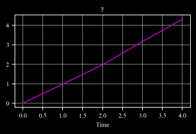
Time histories: [0. 1. 2. 3. 4.]Y values: [0. 0.97952923 1.9754797 3.16437906 4.30533173][ ]:
# TODO: Plot y over time

s.plot( #   'y'
)
Expected figure:
Scale Data#
Assume that y is given in units of [km] and we want to scale it to units of [m] (i.e. scaling by \(1000\)).
\(\color{cyan}{\textit{Task:}}\) Repeat the two last operations, print and plot y, by scaling data() by \(1000\): data('y', scale = 1000), and scale plot by \(1000\): plot('y', scale = 1000)
[ ]:
# TODO: Plot y histories scaled by 1000
...
Expected results for scaled data: Y values: [0. 979.52923405 1975.47969635 3164.37905697 4305.33173132]
[ ]:
# TODO: Plot y over time scaled by 1000
Expected figure: As earlier with y values scaled by 1000.
\(\color{cyan}{\textit{Goal:}}\) Familiarize yourself with all the data operations of the state objects: State object data operations
Parameters#
\(\color{cyan}{\textit{Task:}}\) Define a mass parameter, print its value. Modify it. Store the parameters before and after the modification. Retrieve history values.
[ ]:
# Build on previous s
# TODO: Add a mass parameter

s.mass =                    # 2 # kg

print("System mass:",   # s.mass
)

# TODO: Store the current mass parameter:
s.storeparams(                      # 'mass', t = 0
)

# Modify the mass
s.mass =                    #

# Store the modified mass in different time step:
s.storeparams(                      # ...
)


# TODO: Retrieve mass history:
t_mass, mass_data = s.data(                         # 'mass'
)

print("Modification Times:",                # t_mass
)

print("Mass histories:",            # mass_data
)
System mass: 2Modification Times: [0 1]Mass histories: [2. 5.]Constants#
c4d, then the value of π is given by c4d.pi.[ ]:
# TODO: import degrees to radians constant (d2r)
# from c4dynamics import d2r

phi_deg = 50
phi_rad = phi_deg   # TODO: mutliply by degrees to radians constant

print(phi_deg, "° after conversion to radians:", phi_rad)
Expected: 50° after conversion to radians: 0.8726646259971648
Example 1: Pendulum Simulation#
pend = state(theta = 50 * d2r, q = 0).store the state
write the derivatives of pendulum dynamics: \(dX=\begin{bmatrix} q \\ -(g/L) \cdot sin(\theta) \\ \end{bmatrix}\)
Euler-integrate the derivatives: \(X = X + dX \cdot dt\)
Plot \(\theta\).
Note: use c4dynamics degrees to radians conversion constant to initialize \(\theta\) in radians.
[ ]:
from c4dynamics import d2r

# TODO: set parameters for the pendulum simulation
g =   # 9.81
L =   # 1.0
dt =   # 0.001

# TODO: Define the pendulum object with initial conditions
pend = c4d.state(  # theta = , q =
)

# TODO: Simulation loop
for t in np.arange(  # 0, 5, dt
):
    pend.store(t)
    dX = np.array([  # pend.q, - (g / L) * np.sin(pend.theta)
    ])
    pend.X +=   # dX * dt
[ ]:
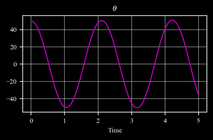
# TODO: plot the angle data scaled back to degrees

pend.plot( # 'theta', scale = c4d.r2d
)
Expected figure:
\(\color{cyan}{\textit{Inline Question:}}\) What’s the disadvantage of the Euler integration we used? what’s its advantage? which other integration methods do you know?
\(\color{magenta}{\textit{Your Answer:}}\) Fill in here.
Example 2: Car Moving in 2D#
\(\color{cyan}{\textit{Goal:}}\) Simulate the \(2D\) motion of a constant-acceleration car.
[ ]:
# TODO: Parameters
dt =   # 0.1
accel_x =   # 0.5

# TODO: Define and store initial
car = c4d.state(  # x=0, y=0, vx=0, vy=1
)
car.store(t=0)

# TODO: Simulation loop
for t in np.arange(  # dt, 5+dt, dt
):
    dX = np.array([  # car.vx, car.vy, accel_x, 0
    ])
    car.X +=   # dX * dt
    car.store(t=t)
[ ]:
# TODO: Retrieve x and y data to plot the trajectory

x_values = car.data(  # 'x'
) # [1] # index 1 to get values without time

y_values = car.data(  # 'y'
) # [1] # index 1 to get values without time [1]
[ ]:
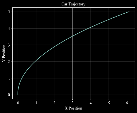
plt.plot( # x_values, y_values
)
c4d.plotdefaults(plt.gca(), 'Car Trajectory', 'X Position', 'Y Position', 12)
Figure Output:
\(\color{cyan}{\textit{Inline Question:}}\) Add \(accel\_y=-0.2\), what’s the trajectory? Explain.
\(\color{magenta}{\textit{Your Explanation:}}\) Fill in here.
Congratulations!#
You’ve completed the introduction to c4dynamics state objects.
Next Steps & Feedback#
Experiment more — try complex systems (e.g., double pendulum, drone with attitude).
Explore the scientific library to learn about the stateful mechanism in filters, sensors, and controllers.
Introduce what you learned to your own system. Replace your arrays with state objects and use the scientific library to develop and test algorithms.
Contribute! — This framework is open-source and community-driven.
We'd love your feedback: Found a bug? Open an issue on GitHub. Want to improve this notebook? Fork the repo, edit, and submit a pull request. Have ideas? Share feature requests or example use cases.
GitHub Repository: c4dynamics/c4dynamics
Upload your completed version of this notebook there (or link it in an issue) and tell us what worked, what didn’t, and what you’d like to see next!
Your input helps make c4dynamics better for everyone. Thank you for learning with us!
Notebook created for educational purposes. c4dynamics © 2025